Lecture 2. How Modern Large Models Work
Lecture 2 · ~100 min · 47 slides
01 · temperature=0 — so the answer is always the same? Yes. → But no.
A simple warm-up question before we start. If you set temperature to zero — will the model's answer to the same prompt be identical every single time?
Intuition says "yes": zero randomness, the model picks the single most likely token, what could possibly go wrong here.
And intuition is almost right. Almost — because in engineering practice, "almost" costs money. Tests that rely on bit-for-bit reproducibility at T=0 occasionally fail for no apparent reason — and the cause isn't your code or your infrastructure, it's something deeper, baked into how computation works on a shared server.
Today we're going to unpack where this "well yes, but actually no" comes from — and a handful of other spots where intuition about models works nine times out of ten, and on the tenth breaks in a predictable, explainable way. We'll walk the inference pipeline from text to answer, and at every stage we'll look at where observation-based intuition stops being a reliable map.
Let's move to the cover slide.
02 · Lecture 2. How Modern Large Language Models Work
Lecture two: how a large language model works on the inside. Today's formula is simple: if you already work with models daily, you'll refresh the fundamentals and pick up some subtleties; if this is your first time, you'll get everything you need.
03 · Lecture map — 7 sections
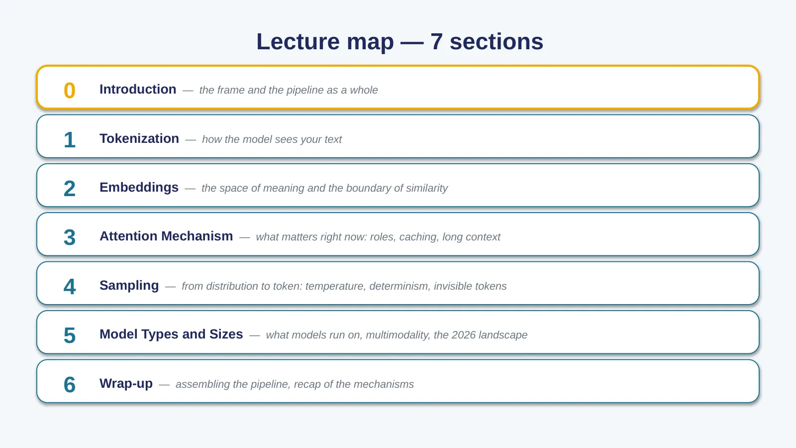
The lecture runs along the inference pipeline: the order of sections mirrors the order of stages a request goes through. Tokenization, embeddings, attention, sampling — four stages. A fifth section, new in this version of the course, covers model types and sizes. The sixth is the wrap-up.
Keep that map in your head.
04 · Today's object is the 'model' layer from Lecture 1's four layers
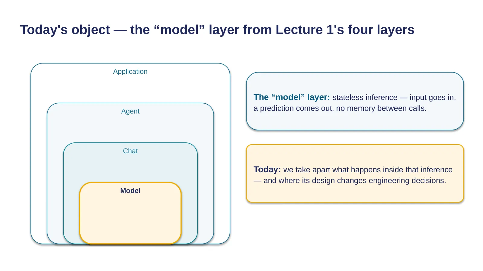
Today's subject is the "model" layer. Lecture one gave us a layered picture: the model at the bottom, chat above it, the agentic loop above that, the application on top. There, the model was described as stateless inference: data goes in, a prediction comes out, no memory between calls. From there we're carrying over, as given, the context window and Pearl's three levels of causality.
With that description we already know how to talk about where the model sits inside the larger system. But the question of "what happens inside that function" — lecture one left that as a black box.
Today, we open that box — everything inside a single layer, the bottom one. Chat, agents, applications — that's lecture three and beyond.
We're chasing boundaries: places where the model's internal design changes how you build prompts and make decisions. Every mechanism was chosen because it has an observable engineering consequence.
05 · Lecture goal: examine how a language model works — and unpack the details that change engineering decisions
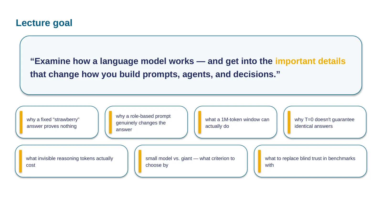
The goal of this lecture: look at how a language model works — and get into the details that change how we build prompts, agents, and decisions. We'll walk the inference pipeline from text to answer, and at every stage we'll show its limits.
We'll show where tokenization breaks arithmetic and why a "fixed" strawberry proves nothing. We'll show why the role in a prompt genuinely changes the answer. We'll dig into why T=0 doesn't give you reproducibility. We'll add the cost of invisible reasoning tokens, a criterion for picking a model by size — and what to use instead of blind faith in benchmarks.
Seven lines under the goal — one per section: by the end of the lecture, each one gets an answer grounded in a concrete mechanism, not intuition.
06 · Data flow in an LLM: words → tokens → vectors → LLM → vectors → tokens → words
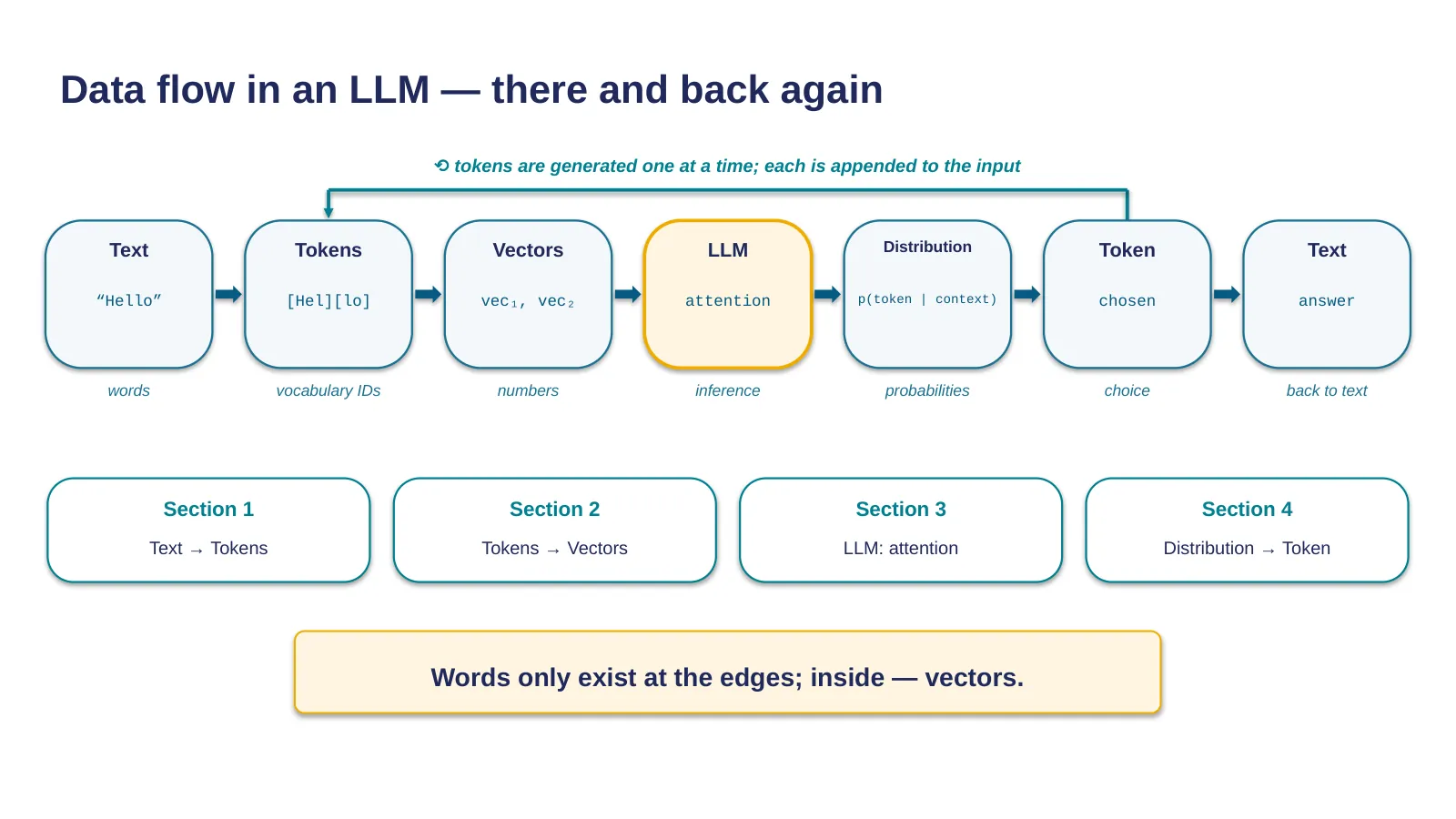
This is the reference diagram for the whole lecture — the inference pipeline, the path of a single request from text to answer. Let's look at it whole, before we dive into any one part; we'll come back to it every time we enter a new section.
On the left is your text. The first transformation is tokenization: the text is cut into tokens, identifiers from the model's vocabulary; that's section one. Next, each token turns into a vector — a list of numbers the neural network can actually compute with; that's section two. In the center is the model itself: the attention mechanism decides which parts of the context matter for the next step; that's section three. On the output side, the model doesn't produce an answer — it produces a probability distribution over the entire vocabulary; one token is picked from it, glued onto the context, and the cycle repeats; that's section four. The last step is assembling the chosen tokens back into text.
The key observation: words only exist at the edges of the pipeline — on the way in and on the way out. Everything inside is operations on vectors. And notice the loop in the diagram: tokens are generated one at a time, each chosen token gets appended to the input — and the pipeline runs again from the top.
This axis isn't just for today — we'll come back to it across the rest of the course. RAG is about managing what makes it into the context before the pipeline runs; agents are a loop wrapped around the pipeline; cost optimization is the economics of the pipeline. Today's lecture moves along this same axis — each section unpacks its own stretch of the pipeline together with where it stops working.
Moving to section 1.
07 · Section 1 — Tokenization: how the model sees your text
Section 1 of 6 — Tokenization: how the model sees your text. The text isn't cut by letters or by words, but by tokens. Next: where the cut diverges from structure — from strawberry to glitch tokens.
The section's general principle: every tokenization quirk has a mechanism, and every mechanism has a testable engineering consequence.
08 · A token is an id from the model's vocabulary. Not a letter and not a word; a statistically frequent subsequence
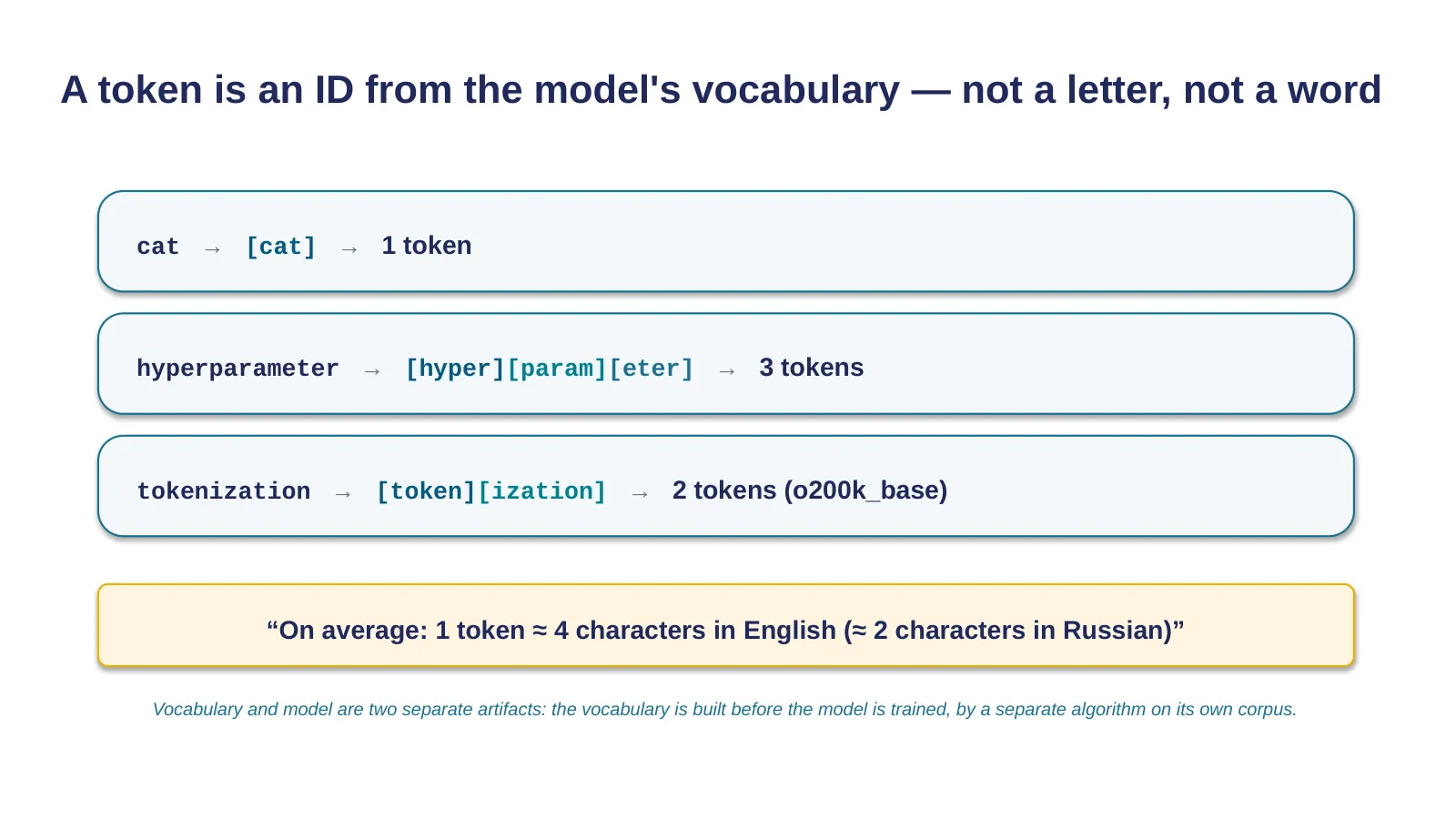
Let's pin down the exact definition. A token is an identifier — an integer from the model's vocabulary; the vocabulary is fixed at training time and doesn't change at inference time. A token isn't a letter or a word — it's a statistically frequent subsequence of characters, learned from a corpus. The common English word cat lands in the vocabulary as a single whole token; tokenization splits into two tokens; the Russian word for "strawberry" splits into three, in that same o200k_base vocabulary.
Vocabulary size in current models runs to hundreds of thousands of entries. A useful cost rule of thumb: one token is roughly four characters of English text and roughly two characters of Russian.
One nuance that often gets lost: the vocabulary and the model are two separate artifacts. The vocabulary is built by a separate algorithm on its own corpus before the model is trained; the model then learns to work with that vocabulary on its own corpus. This decoupling is the source of a whole class of effects we'll come back to in this section.
And the answer to a fair question: why not just work character by character? It's the economics of length. A character-level representation lengthens the input three- to five-fold, and the cost of attention grows quadratically with length — four times longer input means sixteen times more expensive attention layer. Tokenization, warts and all, is a deliberate trade-off that was bought on purpose — not an oversight that will be "fixed in the next version."
09 · BPE is a compromise between an alphabet and a full vocabulary; the vocabulary is built once, before training
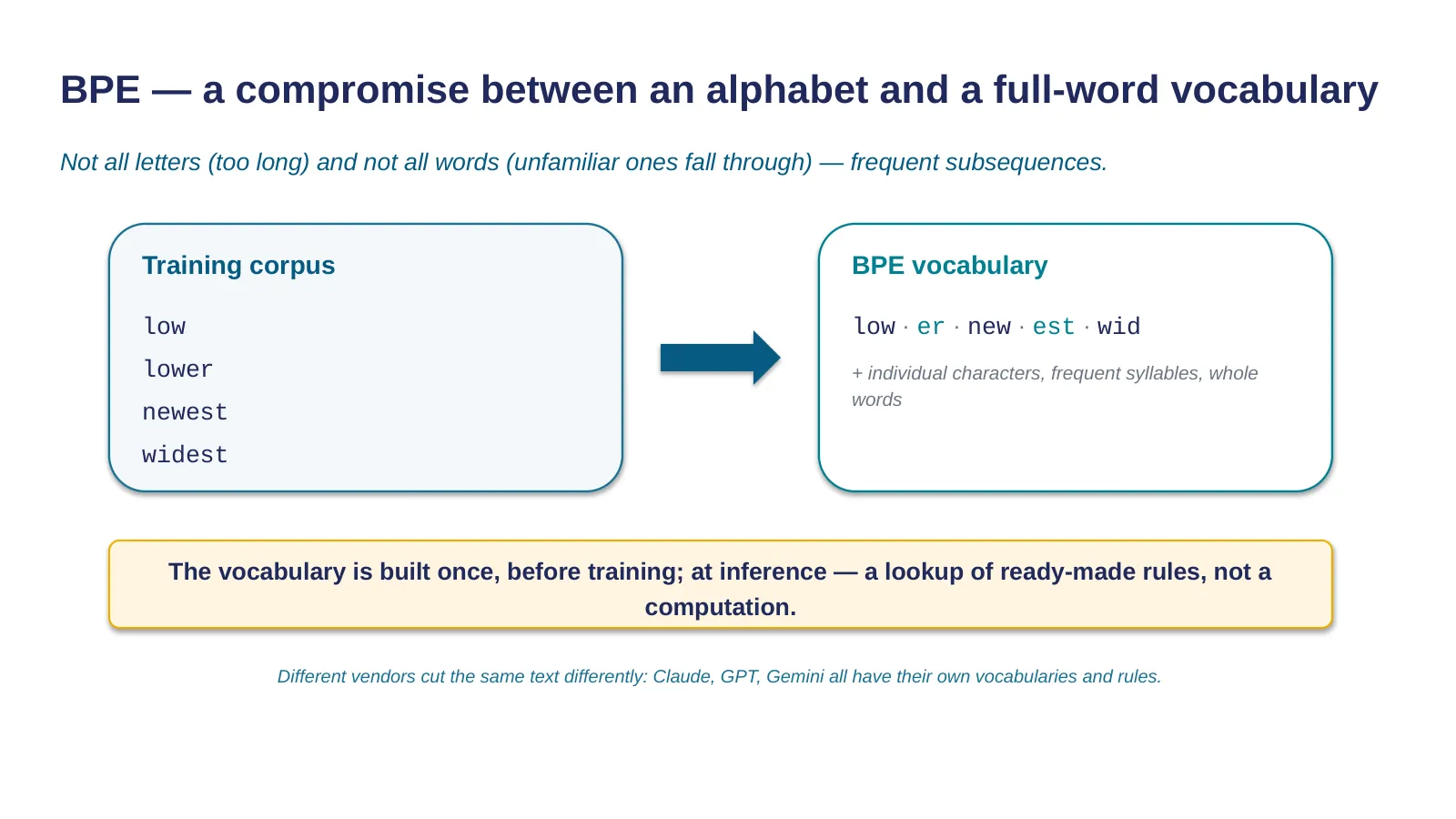
The algorithm behind most modern LLM vocabularies is BPE, byte-pair encoding, and let's unpack it as a compromise between two extremes. A vocabulary made of individual characters can represent any text, but the resulting sequences are long. A vocabulary made of whole words gives short sequences, but any unfamiliar word — a typo, a neologism, a name — falls outside it. BPE sits in the middle: start with an alphabet, iteratively merge the most frequent pairs of adjacent units.
The key engineering detail: the vocabulary is built once, before the model is trained. BPE runs over a corpus, the vocabulary and merge rules get fixed — and that's it; at inference time, tokenization is a lookup against a ready-made table, taking milliseconds, not a computation.
This gives us two consequences we'll need later. First: the tokenizer cuts along the frequency statistics of its own corpus, and that statistic may not match the structure of your task. Second: since the vocabulary and the model are trained on different corpora, the vocabulary can end up holding entries the model has barely ever seen.
It also matters in practice that different vendors count the same text differently — their own vocabularies, merge tables, whitespace handling. The same document will give a different token count with different providers, which means different cost and different context-window usage. When you move workloads between providers, recompute your token budget: for OpenAI models, tokenization is emulated locally with the tiktoken library; for open models, with the tokenizers library.
10 · Patch race: strawberry got fixed in April, cranberry only in July; the underlying class of problem remains
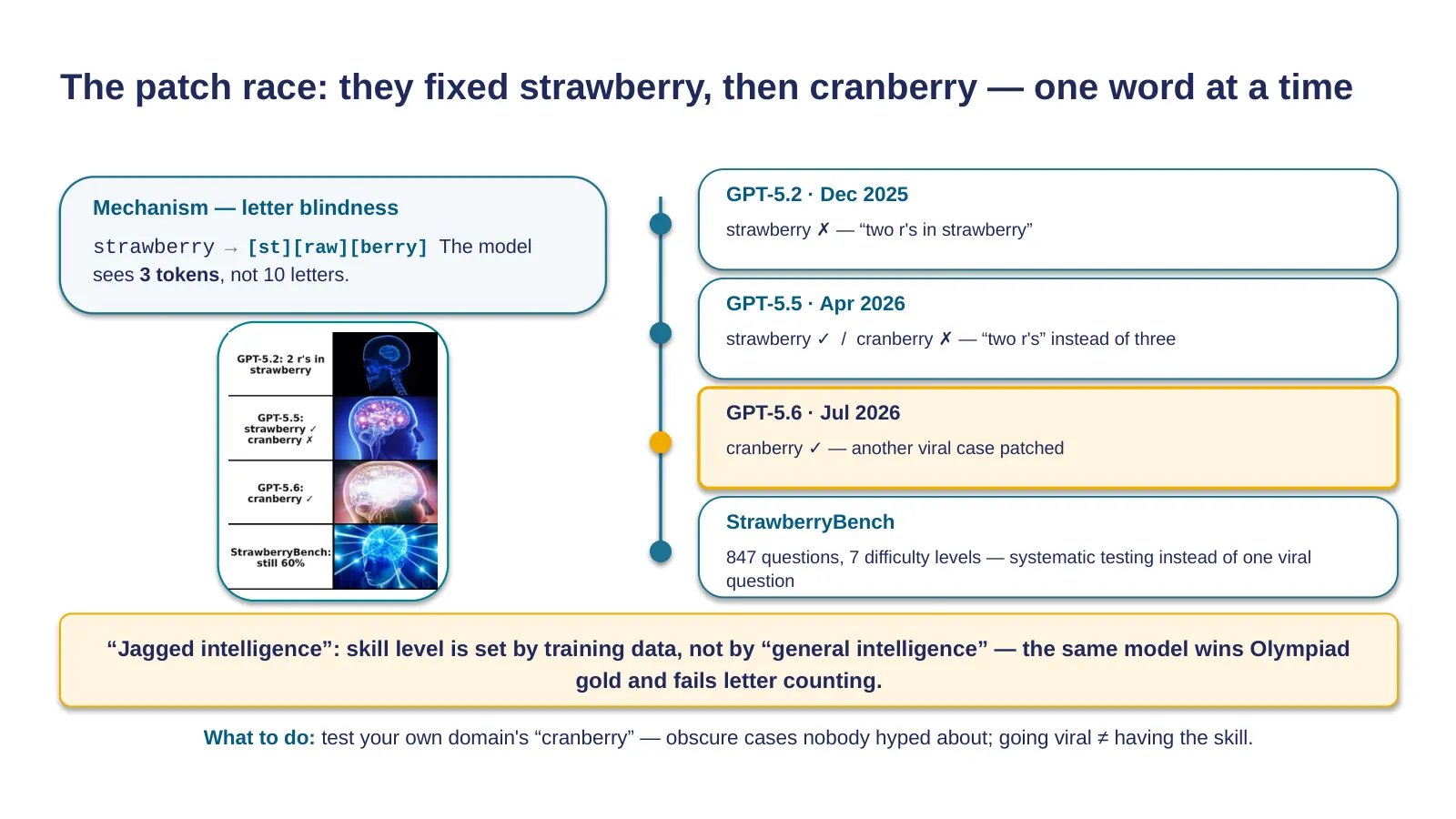
You've probably seen the "how many r's in strawberry" meme — and you probably know that current models get it right. The conclusion "so they've learned to count letters" is false, and here's why.
The mechanism is letter-blindness. The word arrives inside the model as three tokens: ``, not ten letters. Inside a token's learned vector there is no field that says "contains an r at such-and-such position" — what's in there is context statistics. Counting letter by letter requires reasoning on top of the tokenized representation — spelling the word out or calling code; a single forward pass doesn't reliably get you there.
Now look at the 2026 patch race. GPT-5.2, in December 2025, was still answering "two r's" for strawberry. GPT-5.5, released in April 2026, gets strawberry right — but when asked "how many r's in cranberry," it answered "two"; the correct answer is three. And only GPT-5.6, in July 2026, fixed cranberry too — as of when this lecture was prepared; let's check right now on a current model.
Notice the pattern: every viral case gets patched one at a time, in sequence — not by a single across-the-board skill improvement, otherwise fixing strawberry would have closed cranberry too. To check this systematically, StrawberryBench was built — 847 questions across seven difficulty levels; it's there, not in one viral word, that you can see letter counting remains a genuine weak spot.
The phenomenon has a name: jagged intelligence — a capability profile with sharp dips right next to peaks. The same model solves olympiad-level math and fails at counting letters; on multiplication, GPT-4 without tools scored around 59% on three-digit numbers, 4% on four-digit numbers, and 0% on five-digit numbers.
Carry the lesson into practice: if a model passes your test, check it against "the cranberry of your own domain" — a structurally analogous but non-famous example. Passing a viral case is not a skill. And for letter-level operations and arithmetic — reach for an external tool, not a raw forward pass.
11 · The tokenizer cuts by frequency, not by structure: numbers get chunked in groups of 3 digits, code gets cut by whole indentation blocks
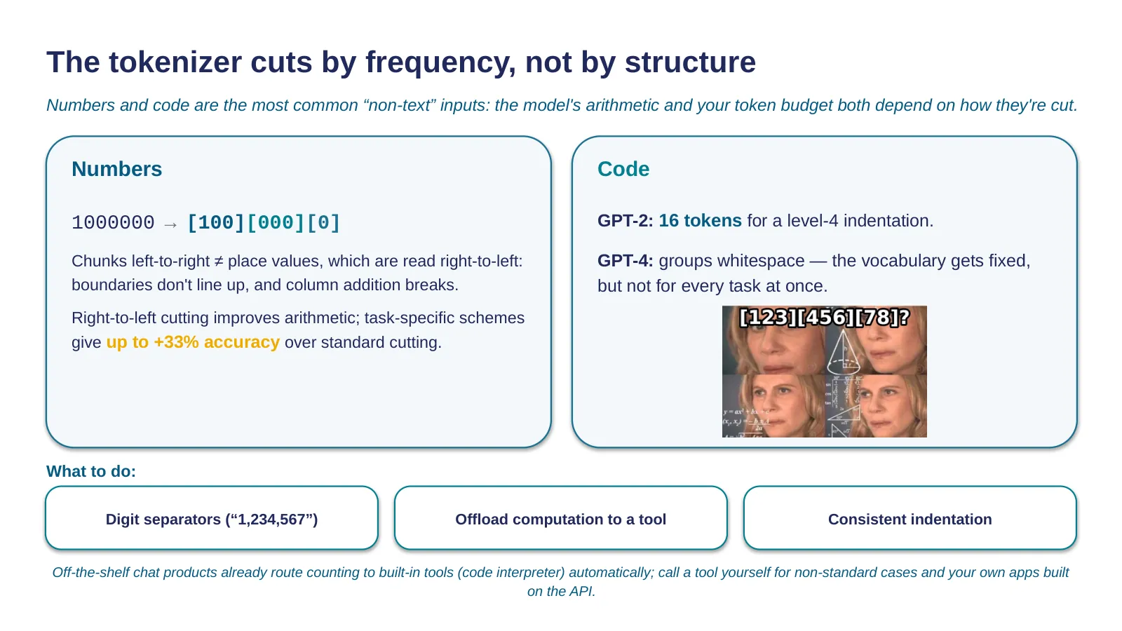
Why an engineer needs to know how numbers and code get sliced up: these are the most common "non-text" inputs, and how they're cut directly determines the model's arithmetic and your token budget.
Numbers. The cl100k_base tokenizer standardized number-slicing into chunks of three digits from left to right: a million turns into groups whose boundaries don't line up with place value. Humans read digit groups right to left — thousands, millions; the model gets irregular blocks, and that's a direct source of some arithmetic errors. Forcing right-to-left slicing measurably improves numerical reasoning, and task-specific number-tokenization schemes have delivered up to plus thirty-three percent accuracy on large-number arithmetic.
Code. GPT-2 encoded every indentation space as its own separate token: a line four levels deep spent sixteen tokens on indentation alone. GPT-4-generation tokenizers group whitespace into single tokens. This is a rare case where a tokenization problem actually got fixed by changing the vocabulary — a useful contrast to strawberry: you can optimize a vocabulary for one common class of input, but you can't make the cut match the structure of every task at once.
Four takeaways. Write significant numbers with digit-group separators. Route any arithmetic beyond a rough estimate out to a tool. For code, use consistent formatting. And an important caveat for practice: in ready-made chat products — ChatGPT, Claude's web interface — counting already gets automatically routed to a built-in tool like a code interpreter; what we just went through becomes critical specifically when you call the model through the API directly, in your own applications and agents, where there's no such automatic routing.
12 · Roughly 4% of the vocabulary is glitch tokens: the vocabulary is built separately from the model, and some entries end up undertrained
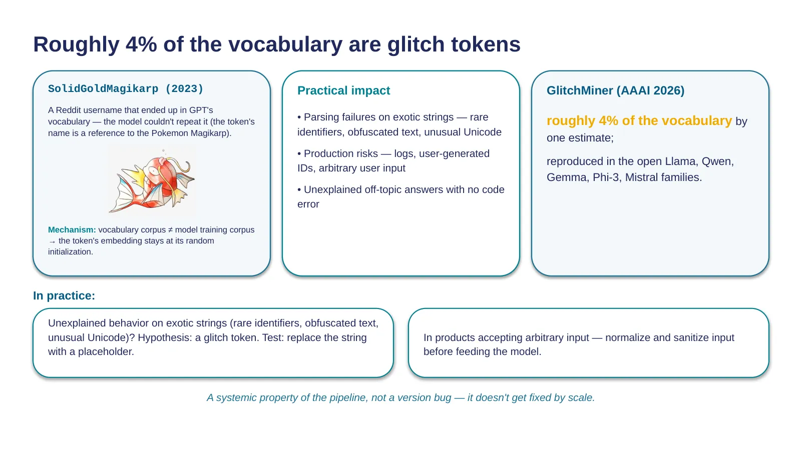
In January 2023, researchers studying clusters in the embedding space of GPT models stumbled on a group of odd vocabulary entries — strings like SolidGoldMagikarp: Reddit usernames that ended up in the tokenizer's training corpus during data collection. Models behaved strangely on these tokens: they couldn't repeat them back, gave off-topic answers, wandered off the subject.
The mechanism, in short: a string can be frequent in the corpus the vocabulary was built on, and earn its own token — while being almost absent from the corpus the model was later trained on. That token's embedding stays close to its random initialization and "means nothing" in the learned geometry.
2026 data tells us this isn't a quirk of the GPT-3 era — it's a systemic property. By one estimate, roughly four percent of vocabulary entries in tested models are glitch tokens; the GlitchMiner framework finds them via gradient search across ten open model families: Llama, Qwen, Gemma, Phi-3, Mistral. The problem reproduces across every family tested — you can't scale your way out of it.
Now — what this actually affects, which matters more than the mechanism itself. First: parsing failures on exotic strings — the model inexplicably loses the thread of a conversation on one specific input. Second: production risk — any system that accepts arbitrary user input is working with a potential source of glitch tokens: logs, auto-generated identifiers, obfuscated text. Third: diagnosis — if behavior is inexplicable specifically on one particular input, "there's a glitch token in there" should be among your hypotheses; it's checkable in a minute by swapping the suspect string for a placeholder. Fourth: sanitize input before feeding it to the model — that filters out not just glitch tokens but a whole adjacent class of tokenization surprises.
13 · The same text in Russian costs ≈2× more tokens than in English; o200k narrowed the gap by a third, but didn't close it
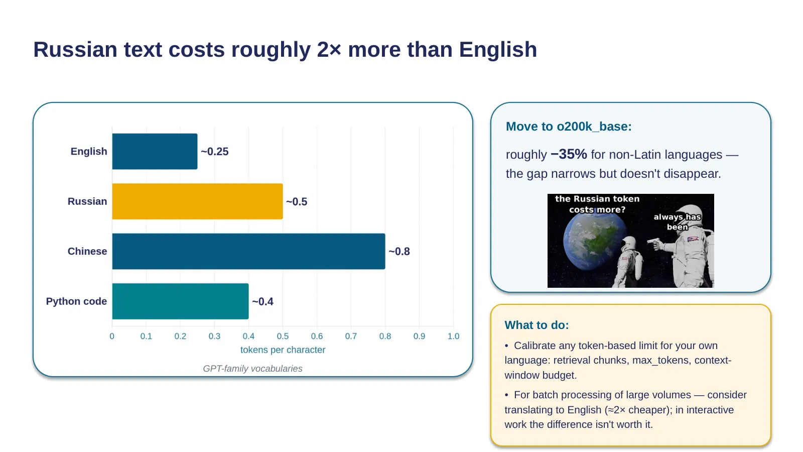
The same text, meaning-for-meaning, costs a different number of tokens depending on the language — a direct consequence of the fact that a BPE vocabulary is trained on a corpus dominated by English. Rough figures: English is about 0.25 tokens per character, Russian about 0.5, Chinese about 0.8, Python code about 0.4. Net effect: a Russian-language request costs roughly twice as much as an English one, and it burns through the context window twice as fast.
The 2024–2026 trend: OpenAI's move to o200k_base cut the per-unit cost of non-Latin-script languages by about 35% — the gap is narrowing, but it hasn't closed. Models with a larger share of Russian in their vocabulary — YandexGPT, GigaChat — show a smaller gap.
The language coefficient leaks into places people forget to check. Chunking documents for search is configured in tokens: a "512-token" chunk holds half as much meaning in Russian, and thresholds copied from English-language guides are systematically too small for a Russian-language knowledge base. The max_tokens limit is the same story: a Russian answer runs longer in tokens, and mid-sentence cutoffs happen more often. Calibrate every token-denominated numeric parameter on your own language and your own data — don't carry it over from someone else's examples.
Moving to section 2.
14 · Section 2 — Embeddings: the space of meanings
Section two of six — Embeddings: the space of meaning. Tokens became identifiers; but a neural network can't compute with an ID number. The second stage turns them into vectors. Let's unpack the three lives of the term "embedding" and find the section's one, but important, gap — the boundary of similarity.
15 · Every token is mapped to a vector from an input lookup table; it's learned during training and then fixed
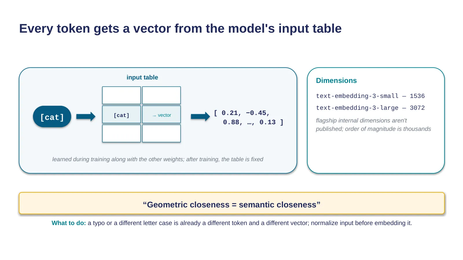
A token is an identifier from the vocabulary, but a neural network can't do anything meaningful with the number 48213. An embedding — a vector representation — is a fixed-length vector assigned to every token in the vocabulary, learned during training together with the rest of the weights. Once training is done, the input lookup table "token → vector" is fixed; at inference time, the model just does a lookup.
The key property of the learned space: geometric closeness corresponds to semantic closeness. "Cat" sits close to "dog," "SSL" sits close to "HTTPS" — not because someone labeled it that way, but because these words showed up in similar contexts in the training corpus.
And one caveat for anyone who's going to work with vectors by hand. In high-dimensional spaces, concentration of measure kicks in: random points end up at roughly the same distance from each other, and "raw" distances compress into a narrow range. So absolute similarity values aren't very informative on their own — what's informative is comparisons and the distribution of values within your specific task.
16 · Embeddings aren't only an internal part of inference: search and RAG run on a separate embedding model
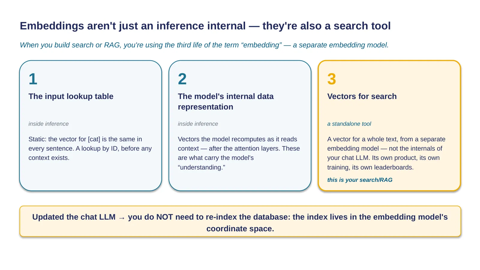
Embeddings aren't just used at inference time — they're also a standalone search tool. Let's unpack the term's three lives.
Life one: the input lookup table — a static "token → vector" table at the input to the LLM. The vector for the token "cat" is the same one, in any sentence. Life two: the internal representation of data inside the model. The sequence of input vectors passes through dozens of attention layers, and by the output, each position's vector has been updated based on its surroundings — these representations are what actually carry the model's "understanding." Both of these lives are internal to inference.
The third life is your working tool. When you're building search or RAG, this is the one you actually use: you call an embedding API and get back a vector for a whole piece of text, from a separate model specifically trained for search and comparison. This isn't the inner workings of your chat LLM — the embedding model can come from a completely different vendor, and that's normal practice.
The distinction worth keeping in your head is simple: if you're talking about cost and context window — that's tokens and the input lookup table; if you're talking about "what the model understood" — that's the internal representation of data; if you're talking about search and vector databases — that's the output embeddings of a separate model.
And the standard mix-up mistakes. "We already have a subscription to a chat model — why pay for an embedding model too?" — because the chat model doesn't hand you search vectors. And the mirror image: "we upgraded the LLM — time to reindex the database" — no you don't; reindexing is needed exactly when the embedding model itself changes.
17 · Embedding space has hundreds to thousands of dimensions; tokens close in meaning sit near each other
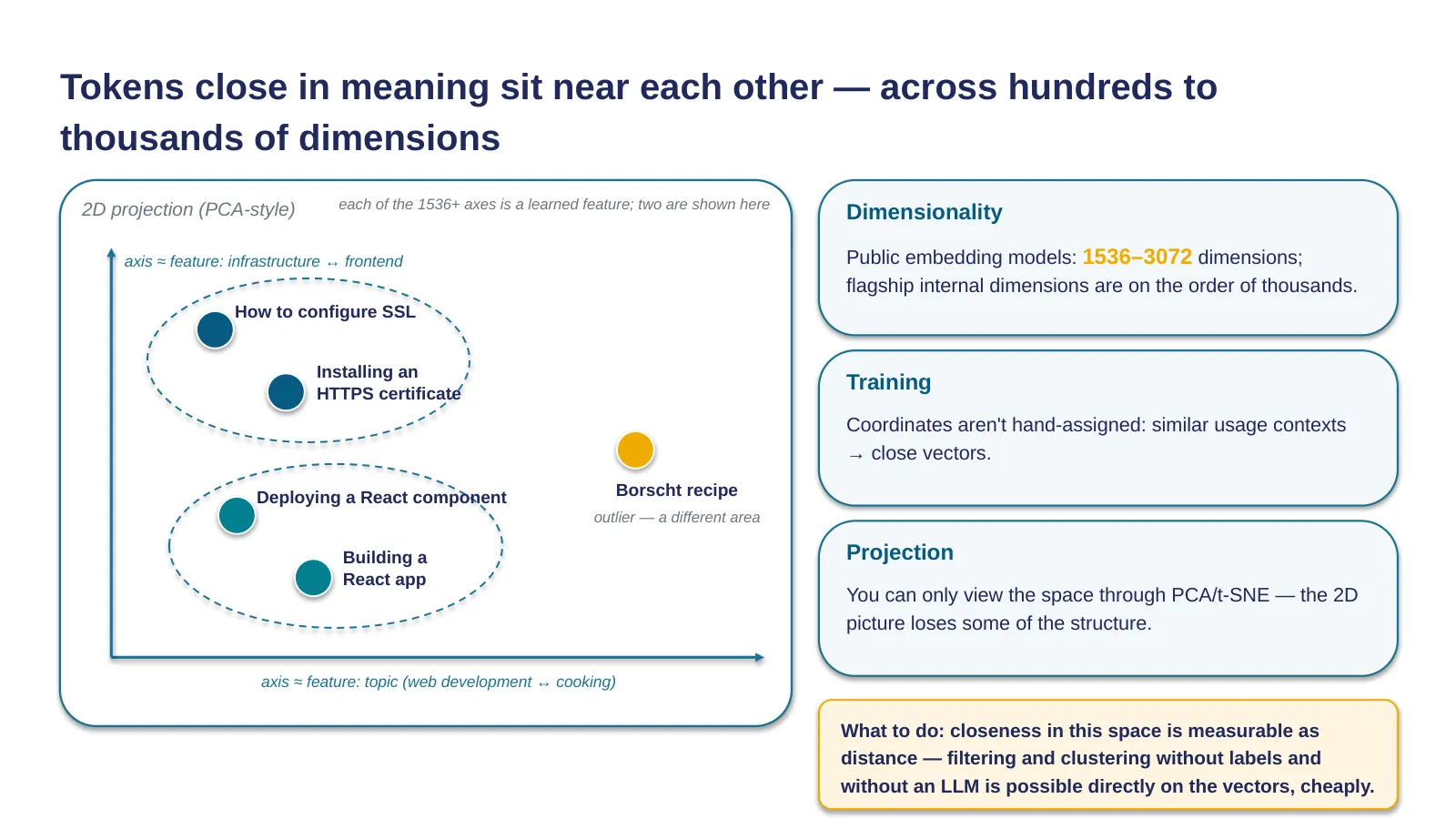
How the space where these vectors live is structured. Every point is a token or a piece of text; the coordinates are hundreds or thousands of numbers. The meaning of each dimension isn't assigned by hand — after the fact, many of them read as recognizable features: topic, formality, domain.
Take a look at the picture — a two-dimensional projection: two semantic clusters and an outlier. "How to set up SSL" and "Installing an HTTPS certificate" are surrounded by the same words — so their vectors end up close together; "Deploying a React component" and "Building a React app" sit next to frontend-related words; and "Borscht recipe" lives in a completely different region — a lone outlier among technical texts.
Remember this is a simplification: the real space has thousands of dimensions, and any flat projection loses part of the structure.
And let's repeat the caveat, because it costs real money in practice: an absolute similarity value doesn't tell you much on its own. What works is comparisons — "this document is closer than that one" — and the distribution of values in your specific task. There's no universal threshold like "above 0.8 means similar."
18 · High similarity means 'about the same thing' — not 'the same meaning': similarity ≠ relevance
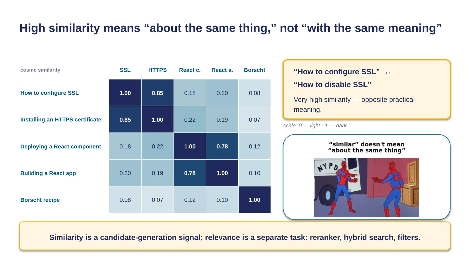
First — proof that similarity actually works. Five short texts, a pairwise cosine-similarity table: task-synonymous pairs — "set up SSL" and "installing an HTTPS certificate" — score around 0.85; topically related React texts — around 0.78; borscht against anything technical — 0.05–0.15. A search for the Russian word for "strawberry" finds documents about strawberries and wild strawberries with no synonym table at all — that's what embeddings give you on top of full-text search.
Now — the boundary, and this is new material even for people who actively build semantic search. High cosine similarity means "about the same thing" — not "about the same thing with the same meaning." The pair "how to enable SSL" and "how to disable SSL" gets a very high similarity score: same topic, same vocabulary, same syntactic frame — and the practical meaning is the opposite. An embedding averages the contextual statistics of the whole text; a short negation shifts the vector only weakly.
In production this looks painful: a user asks how to turn on certificate verification, search confidently surfaces an article on how to turn it off, the LLM in the RAG pipeline dutifully summarizes it — and a system with great similarity metrics hands out harmful advice.
The engineering answers are well known: a reranker, a second model that scores the query-document pair as a whole; hybridizing with full-text search for exact terms; filters and metadata for directional attributes. And a diagnostic trick: build a validation set of pairs with deliberate traps — on/off, before/after, different versions — and see what comes out on top.
The full design of a RAG pipeline is lecture three; what we take from here is the principle: cosine similarity is about topical closeness, relevance is a separate task.
19 · Embeddings are the foundation of understanding an LLM: the model operates in vector space, not in strings
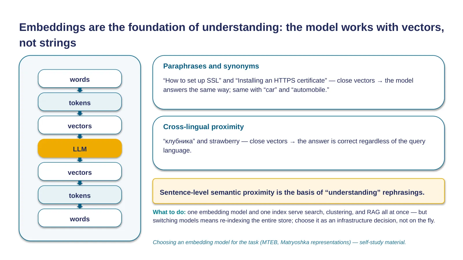
Let's wrap up the section. The model doesn't work with words — it works with vectors; words only exist at the edges. This explains "understanding": "how to set up SSL" and "installing an HTTPS certificate" get a similar answer because they land at nearby points in the space. Same story with cross-language closeness: the Russian word for "strawberry" and the English word "strawberry" are close vectors.
On the practical side: similarity search, clustering, and semantic search with RAG all run on the same vectors. One embedding model and one index serve several functions at once, which makes the choice an infrastructure decision — and switching is expensive: reindexing the entire store. And remember: there's no inverse operation — you can't recover text from a vector.
How to choose an embedding model for a given language — I'll leave that for self-study.
Moving to section 3 — the densest part of the lecture.
20 · Section 3 — Attention Mechanism: how the model decides what to rely on in the context
Section three of six — The attention mechanism, the densest part of the lecture. Everything grows out of this: why chat gets cached, why the role changes the answer, what a million-token window can actually do. We'll go through the attention matrix, the KV-cache, caching economics, role, and the window race.
21 · Attention is checking every token against every other token: N × N at each step
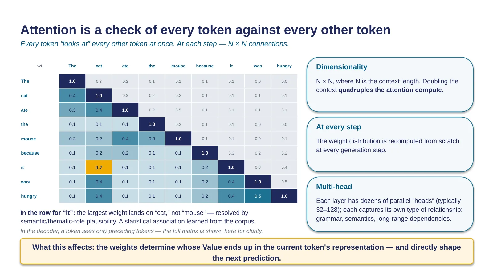
You know the word "attention" from every other transformer paper; let's pin down its exact shape. Attention is a matrix operation: every token in the context is compared against every other token, and for a context of length N, the weight map is N by N.
From here comes the architecture's main economic property: doubling the context quadruples the amount of attention computation. When we get to the cost of million-token windows — this is exactly where the root of it lives.
On the slide is a simplified seven-by-seven matrix for "The cat ate the mouse because it was hungry." In the row for "it," the largest weight sits on "cat," not on "mouse" — the pronoun resolves to the animate subject of the same... well, in this case it's resolved by which noun is the more plausible subject of "hungry." Technically this is a statistical association learned from the corpus, not a grammatical parse.
The real mechanism is multi-layered: at every layer, dozens of "heads" work in parallel, typically 32 to 128, each specializing in its own type of relationship.
What matters most is what the weight distribution actually affects. The weight of each connection determines how much of that token's Value vector flows into the final representation of the position. And that position's representation is exactly what the next prediction gets built from. Attention weights directly determine the next token.
22 · Attention outputs a weight distribution over every token in the context — mechanically via three projections, Query/Key/Value
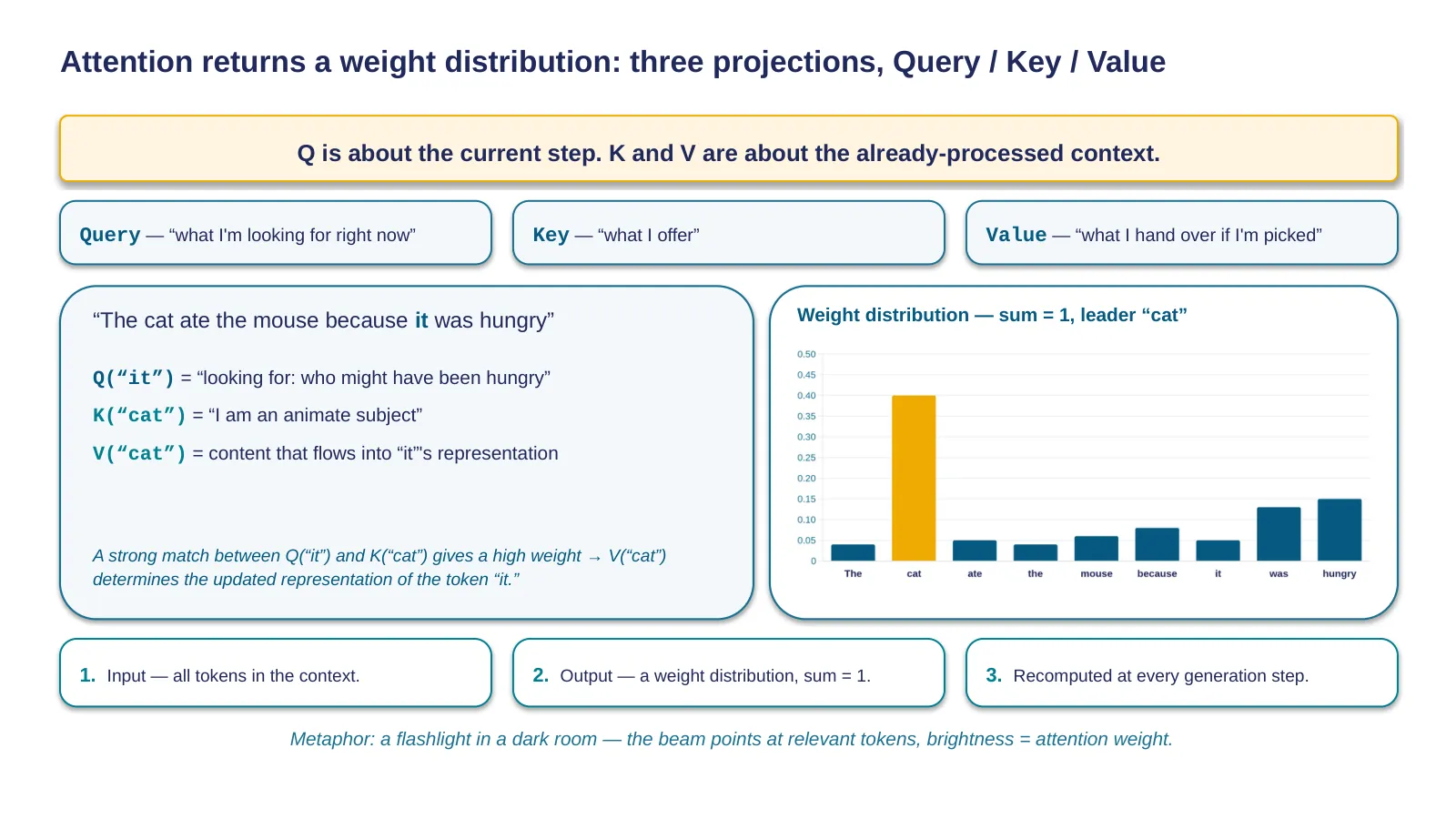
Let's pin the definition down precisely. The working metaphor is a flashlight in a dark room: every token is present, but the beam points at the relevant ones, and brightness is the weight. At every step, attention returns a weight distribution over the entire context, the weights sum to one, and it's recomputed from scratch every single time.
Now — one level deeper, on our sentence. For every token, the model computes three projections: Query, Key, Value. Take "it." Its Query reads roughly as "looking for: who might have been hungry." The token "cat" offers up its own Key — "I am an animate subject" — a business card by which other tokens' queries find it. When the Query from "it" and the Key from "cat" match well, the weight comes out high. Then the Value of "cat" kicks in — the content that actually flows into the representation of "it."
In plain terms: Query is the token's question; Key is what it uses to answer other tokens' questions; Value is what it hands over if it gets picked.
One thing is worth remembering: Query is about the current step, while Key and Value are about the already-processed context, which doesn't change. That asymmetry is where the entire inference industry's central optimization comes from — we'll see it on the next slide.
23 · K and V for the context are cached; only Q is recomputed — hence the two generation phases and 'long chats slow down'
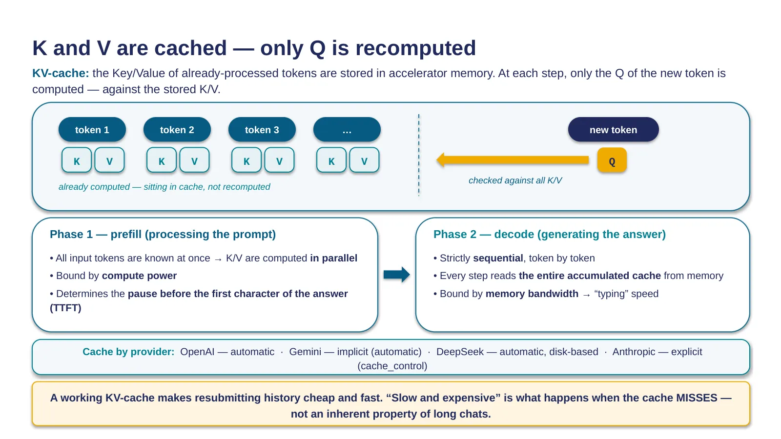
Recall the observation from the last slide: Query is about the current step, Key and Value are about the already-processed context. Generation is autoregressive: tokens come out one at a time, and a naive implementation would recompute K and V for every token from scratch at every step — but they don't change. This gives us the central optimization of all large-model inference: the KV-cache — the Key and Value vectors of already-computed tokens are stored in accelerator memory, and at each step only the Q of the new token gets computed.
Out of the cache comes an asymmetry between two phases. Prefill — processing the input prompt: all tokens are known at once, their K/V get computed in parallel; this phase is compute-bound and determines the delay before the first character of the answer. Decode — generation: strictly sequential, and at every step you have to read the entire accumulated cache from memory; this phase is memory-bandwidth-bound and determines typing speed.
The precise wording of the conclusion matters here, because it easily gets distorted into the folk wisdom "new task, new chat." As long as the KV-cache is working — that is, the history matches what's already been computed — resubmitting that history is cheap and fast: that's the entire point of the cache existing. "Slow and expensive" isn't a property of long chats in general — it happens specifically when the cache misses: when the context changes near the start, when the session has expired, when the provider has evicted your cache from memory to make room for someone else's load.
Cache implementation differs by provider, and that directly affects what we have to do by hand. At OpenAI and at DeepSeek, the cache kicks in automatically; DeepSeek's is even disk-backed. Google Gemini has implicit caching, also on by default. Anthropic's cache is explicit: you need to place a cache_control marker yourself — as of when this lecture was prepared. The practical takeaway: if you're on Anthropic and you're not seeing savings, check whether the marker is placed where it needs to be; for the other three, check the cache-hit-rate metrics in the API response.
Scale of the effect: at context lengths of hundreds of thousands of tokens, one user's cache occupies gigabytes of accelerator memory — hence providers' aggressive batching and the premium price on long contexts.
24 · Prompt caching is a bet on reuse: reads cost 0.1× the base rate, writes cost more than plain input, and one changed token invalidates everything after it
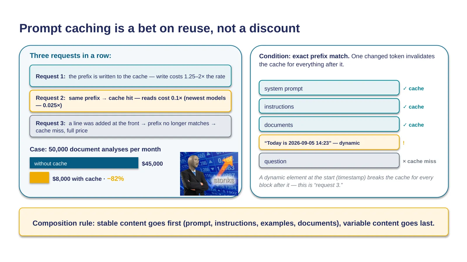
The KV-cache lives inside a single generation. Providers took the next step: if two different requests share an identical prefix — the same system prompt, instructions, documents — its K/V can be reused across requests. This is prompt caching, and since 2025–2026 it's been the single biggest lever for optimizing the cost of LLM workloads.
Let's trace the mechanics through three consecutive requests — it's easier to see this way than through isolated numbers.
Request one: you send the prompt for the first time, there's no cache yet — the prefix gets written into the cache, and that write costs more than a normal input, anywhere from 1.25 to 2 times the base rate. Request two: you send the same prefix — a new user question at the end, but the same system and documents — the prefix matches byte-for-byte, the cache hits, and you pay a tenth of the base rate, on the newest models as little as one-fortieth. Request three: someone added a single line to the top of the prompt — say, the current date — and now the prefix no longer matches. The cache misses: the whole request pays full price, as if the cache never existed.
The cache isn't free — it's a bet on reuse: it pays off from the second or third hit onward. The scale of the effect is real: one case involving 50,000 document analyses a month went from $45,000 without the cache to $8,000 with it — an 82 percent saving.
The key technical condition is exact prefix match: the cache only fires if everything up to the checkpoint matches byte for byte. The classic self-inflicted wound is putting something variable at the start of the system prompt, like the current date and time.
From this comes a rule of composition: stable content goes first, variable content goes last. And here's a one-minute audit for a live pipeline: look at the cache-accounting fields in the API responses — if cache reads are zero despite a stable system prompt, you can almost certainly fix it in one evening by reordering the prompt. For multi-step agents, the cache isn't an optimization — it's a condition for being profitable at all; we'll come back to this in the next lecture.
25 · A role works through attention weight: role tokens shift the distribution, but don't raise the model's actual quality
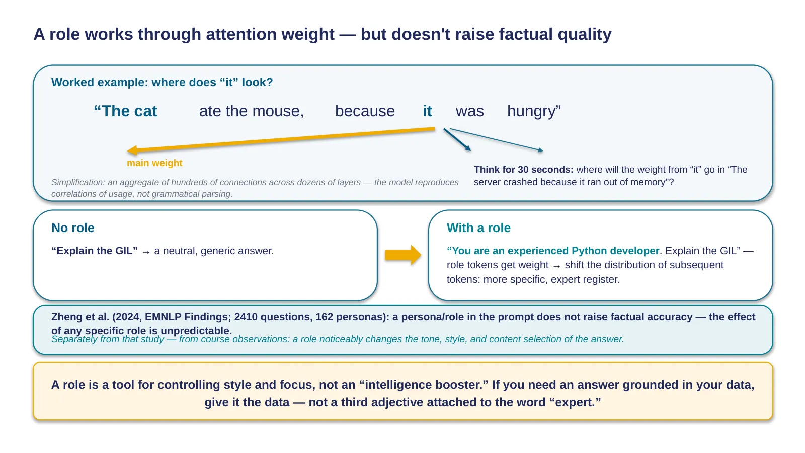
Let's stretch our legs for a second: "The cat ate the mouse because it was hungry." By the time the model reaches the token "it," it resolves who "it" refers to — and we've already seen that the weight leans toward "cat." The model isn't doing a grammatical parse; it's reproducing usage correlations.
Test your intuition: "The program crashed because it forgot to handle null." Where does the weight from "it" go?
In most models — to "program": the only grammatically plausible candidate, and the statistics of technical text only reinforce that choice.
Now — the reason you already needed to know this. Let's compare two prompts. "Explain the GIL" with no role — the model answers neutrally. "You are an experienced Python developer. Explain the GIL" — you've probably noticed that a prompt like this behaves differently. The mechanism: the tokens "experienced," "Python developer" pick up weight in the attention distribution while generating every token of the answer, and the choice shifts toward what's consistent with them.
And the boundary of the effect, worth knowing before you start overusing roles in prompts: a study by Zheng and colleagues, EMNLP 2024, tested 2,410 questions and 162 roles — a persona in the prompt doesn't improve factual accuracy, and the effect of any specific role is unpredictable. Separately from that study — based on the course's own observations — a role does noticeably change the tone, style, and content selection of the answer, and that's a distinct effect, not the same thing as factual accuracy.
A role shifts the distribution; it doesn't add knowledge. If the model doesn't know the answer, an "expert" role won't make it know — it'll make it sound more confident without being any more correct. If you need an accurate answer grounded in your data, give the model the data, not a third adjective in front of the word "expert."
26 · The 2026 frontier standard is a window up to 1 million tokens; but the 'advertised window' and the 'usable window' are different quantities
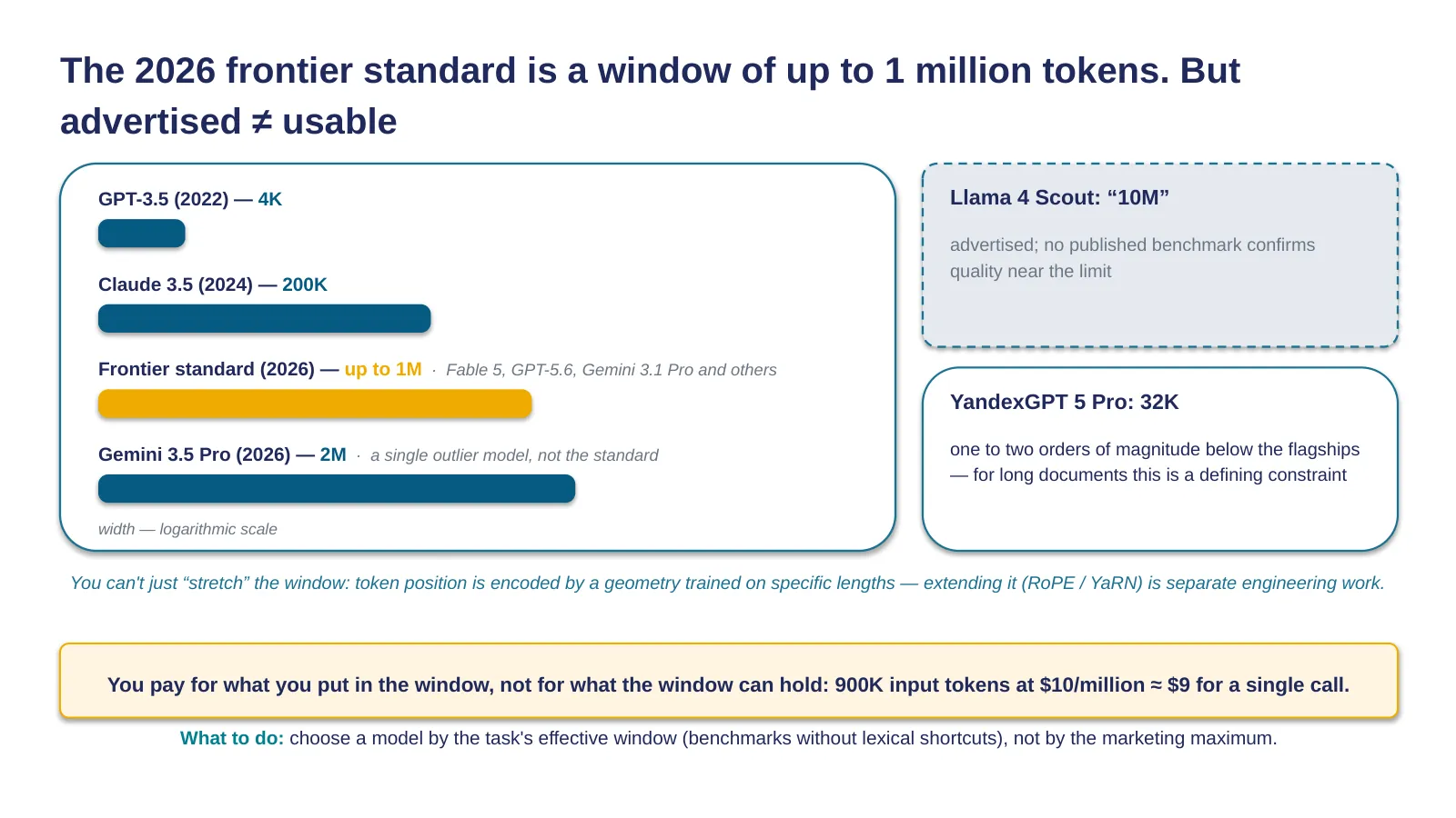
The context window — the maximum number of tokens per request — has grown three orders of magnitude in four years: 4,000 for GPT-3.5 at the moment ChatGPT launched, 200,000 for Claude 3.5 in 2024, and the 2026 frontier standard is up to a million: Fable 5, GPT-5.6, and Gemini 3.1 Pro all hold this level, and for some of these models the full window is included in the standard price with no surcharge.
Two sobering outliers around that standard. Above it: a singular case — Gemini 3.5 Pro holds two million tokens, but that's an exception, not a new standard. Higher still: marketing — Llama 4 Scout claims ten million, but no published benchmark confirms preserved quality anywhere near that limit. Below it: a contrast — YandexGPT 5 Pro works with a 32,000-token window, which is the defining constraint for tasks involving long documents.
Why is the window finite, and why can't you "just make it bigger"? The first reason is familiar: the quadratic cost of attention plus a linearly growing cache. The second is subtler: a token's position is encoded in the model's geometry in a way that was trained on specific lengths, and naively stretching it breaks the mechanism — I'll leave the details in the course materials for anyone curious about the engineering of positional encoding.
And the arithmetic of money. A full window is tokens you pay for as input on every single request: a call to a premium model at $10 per million input tokens, filled to 900,000 tokens, costs about $9 — for one call. The question "how much context does this task actually need" matters more economically than "how much can the model accept."
27 · Verbatim-insertion retrieval is nearly solved — but without lexical overlap, 11 of 13 models lose more than half their accuracy by just 32,000 tokens
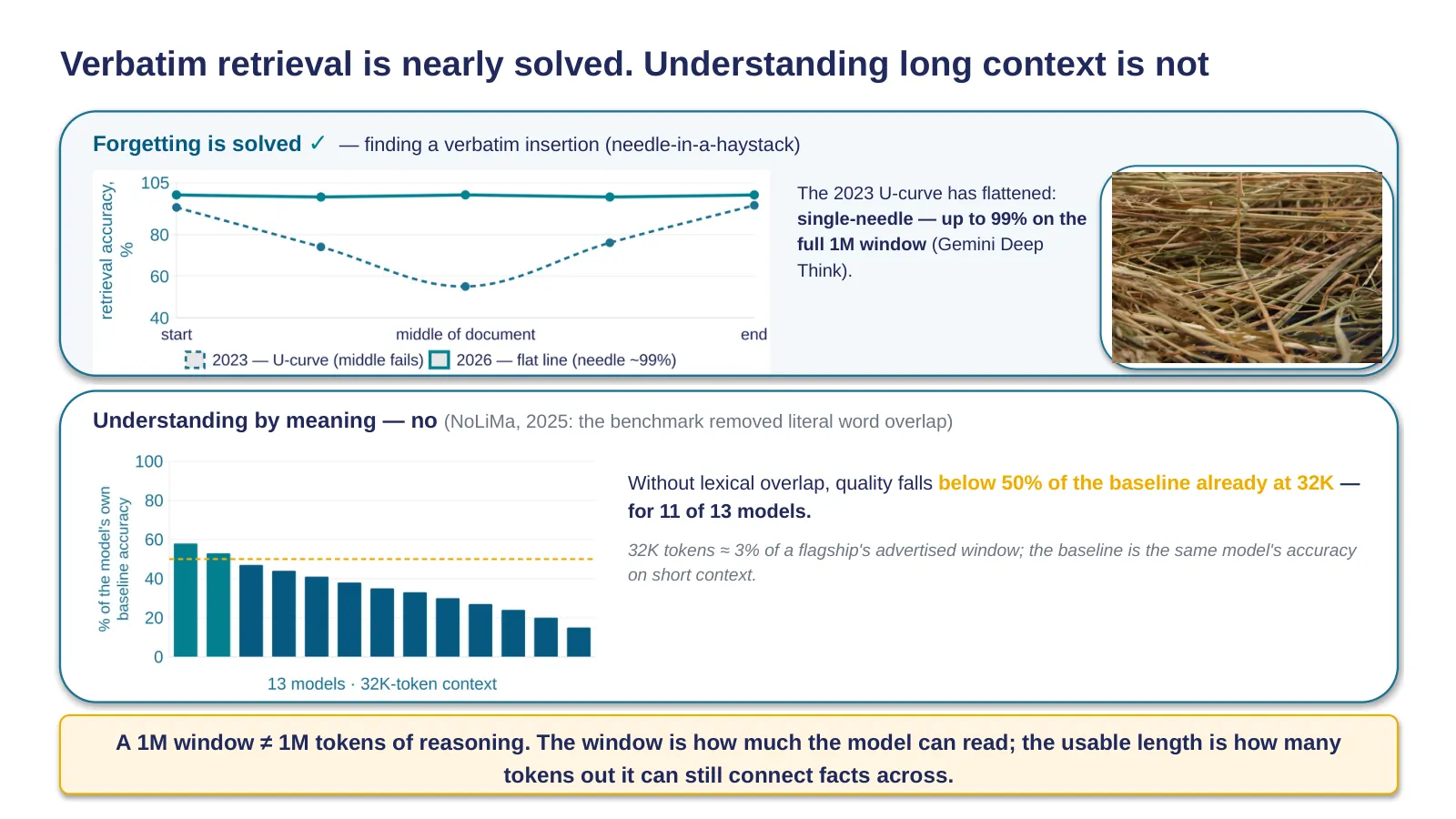
You probably know the classic 2023 result, "Lost in the Middle": a fact buried in the middle of a long context gets retrieved worse than one near the edges. That piece of knowledge needs a 2026 update — in both directions.
The good news: literal "needle in a haystack" search — finding a phrase that was inserted verbatim — is practically solved by the flagships: up to 99% on a full million-token window. If your task is finding where in a contract a dollar figure is mentioned, a large window works almost exactly as advertised.
The bad news came from the NoLiMa benchmark, which removed the main crutch these tests usually lean on — literal lexical overlap between the question and the hidden fragment. When what you're looking for has to be inferred by meaning rather than by matching words, the picture collapses: eleven out of thirteen tested models drop below half of their own short-context accuracy. And this happens already at 32,000 tokens — not at a million, at three percent of a flagship's advertised window.
The U-curve didn't go away — it hid behind impressive numbers from tests that measure retrieval, not reasoning. Notice: the gap between these two tiers isn't a minor benchmarking nuance — it's a direct engineering consequence of what task you're actually paying for when you buy a million-token window.
A formula worth remembering: a million-token window doesn't equal a million tokens of reasoning. The window is how much the model can read; effective length is how many tokens it can still connect facts across without literal cues, and for current models that second number is many times smaller than the first. The consequences: critical instructions go at the start or the end, not in the middle; dumping your entire knowledge base into the window loses to good retrieval with five to ten targeted chunks — more on that next lecture; and test a model at the actual working length of your task, not on a short demo from the vendor's documentation.
Moving to section 4.
28 · Section 4 — Sampling and Generation: how a single token is born out of a probability distribution
Section four of six — Sampling and generation. Three stages down; the result is a probability distribution over the whole vocabulary. The fourth stage is sampling: picking one token, the only part of the pipeline you control directly. Let's test the trickiest of the six claims in this lecture: does T=0 really give you identical answers.
29 · At every step, the model outputs a probability distribution over the ENTIRE vocabulary — then picks one token
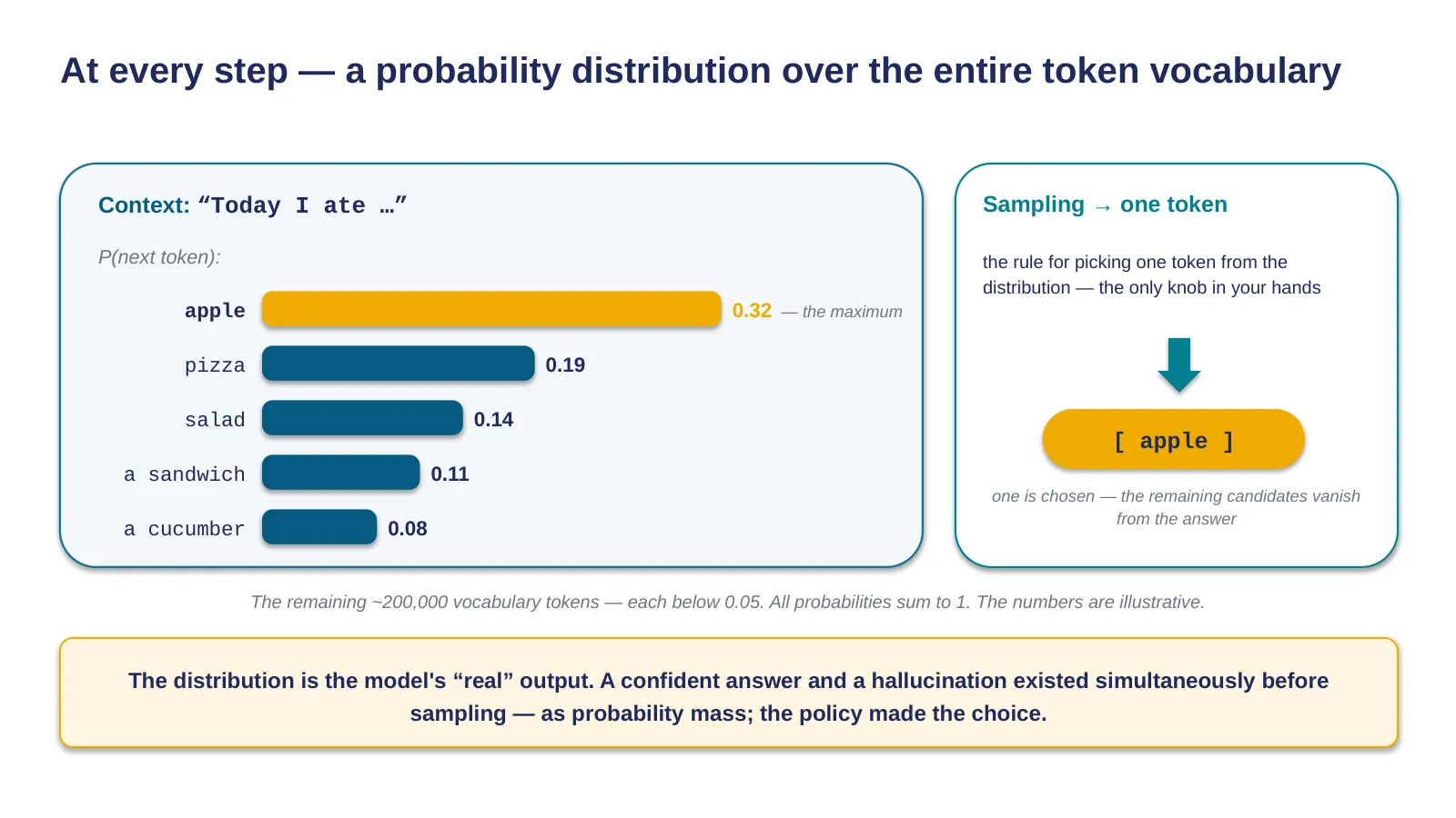
Here's the output of the pipeline's first three stages: a probability distribution over the entire vocabulary — for each of roughly two hundred thousand tokens, a probability of being the next one. For the prompt "Today I ate…" the distribution might look something like: apple — 0.32, pizza — 0.19, salad — 0.14, then a long tail.
Sampling is the rule for picking one token out of that distribution.
It's worth internalizing, once, just how much this distribution is the "real" output of the model, and everything else is a policy layered on top of it. A confident answer and an evasive one, a correct fact and a hallucination, "Paris" and "you might mean…" — before sampling, all of these existed simultaneously, as probability mass spread across different continuations; the choice was made by the policy, not by the model's "opinion."
Practical consequence: some providers expose a slice of this information through the API — log-probabilities of the top candidates at every step. A wide, spread-out distribution on a key token in the answer is an honest signal of model uncertainty that the answer text itself may never reveal. For classification pipelines, this is a cheap way to get a confidence measure without a second call asking "how confident are you" — a second call that, incidentally, would measure not the model's actual confidence but how well-trained it is at answering that kind of question.
30 · Temperature is a logit divisor: it changes how sharp the selection is, not the model's knowledge
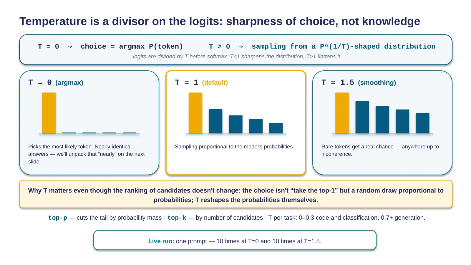
You already know these knobs — let's tighten the mechanics into an exact formula. At T=0, the choice is argmax P(token): deterministically take the token with maximum probability. At T>0, the model samples from a distribution transformed by raising P to the power of one over T — the logits get divided by T before the softmax.
Here it's worth pausing on a question that often causes confusion. The ranking of tokens by probability doesn't change with temperature — the most likely token stays the most likely at any T. So why does temperature matter at all?
The answer is that picking a token isn't "take the top-1 off a list" — it's a random draw, where the probability of picking each token is proportional to its probability in the distribution. And temperature changes those probabilities themselves, not their order: at T below one the distribution sharpens; at T above one it flattens out, and tokens that used to be nearly impossible get a real shot.
Second tier: top-p cuts the tail by probability mass, top-k cuts it by number of candidates. The practice hasn't changed: temperature is the main knob, these two are fine-tuning.
Now, a live run: the same prompt — "come up with a name for a note-taking app" — several times at zero and several times at one-point-five.
The first batch gives near-identical answers — "near" is carrying more weight here than it looks, and the next slide is entirely about that. The second gives a spread from genuinely good finds to incoherence.
31 · T=0 does not give you determinism: on standard vLLM, 80 unique answers out of 1,000 identical requests
This claim is the trickiest of the six we're covering today, because it's almost true, and people build tests and pipelines on top of it. You set temperature to zero, expecting: same request, same answer.
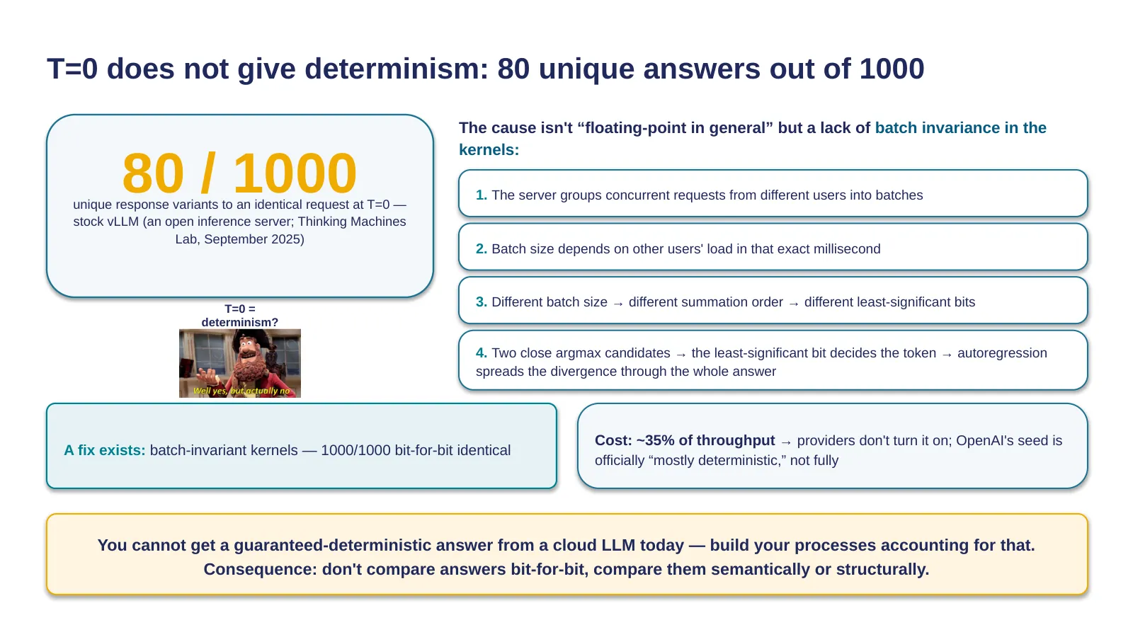
A check on real infrastructure: standard vLLM, a thousand runs of an identical request — eighty unique variants of the answer. Zero really does make the argmax choice deterministic — but the distribution the argmax is taken from turns out to be slightly different from run to run.
The cause runs deeper than the usual "it's just floating point on the GPU." The main culprit is the lack of batch invariance in compute kernels. A provider's server dynamically groups simultaneous requests from different users into batches; batch size depends on the load at that particular millisecond; and many kernels use a different summation order depending on batch size. Floating-point addition isn't associative — and when two argmax candidates are close, the least significant bit decides the token; autoregression then spreads that divergence through the rest of the answer.
Your "deterministic" request is nondeterministic because you're sharing a server with other users, and their traffic changes your batch size.
The most instructive part: the problem is solvable — and the solution has been rejected on economic grounds. Batch-invariant kernels make a thousand out of a thousand runs bit-for-bit identical. The cost is about 35 percent of throughput, which is why providers don't turn this mode on by default; that's also why OpenAI's seed parameter carries the status "mostly deterministic," with no hard guarantee.
Let's state the main takeaway in this order, because the order matters here: you cannot get a guaranteed deterministic answer from a cloud LLM today — this isn't a temporary bug, it's a consequence of an economic choice made by providers, and you need to design your processes with that fact in mind. From that, as a consequence and not as the headline point: don't build tests on bit-for-bit answer comparison — compare semantically or structurally; and if you genuinely need strict determinism, that's a separate infrastructure requirement with a price tag of a third of your throughput.
32 · Alongside the classic 'randomness + length' knobs, a new axis has arrived: 'reasoning depth + verbosity'
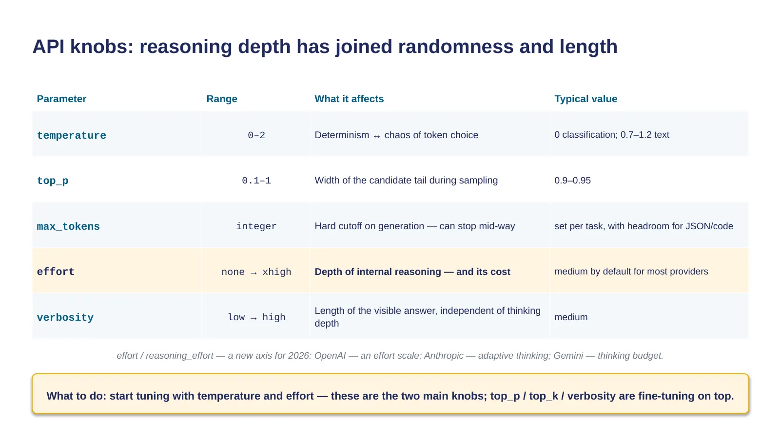
The classic set — temperature, top_p, max_tokens — you already know; the table on the slide fixes the range and the typical value for each.
The 2026 news: reasoning models grew two new knobs, and they control a different axis. Effort, or reasoning_effort, is the depth of internal reasoning: OpenAI has a scale from "none" to "xhigh," Anthropic has an effort parameter, Gemini has a thinking budget. Verbosity is the length of the visible answer, independent of reasoning depth: you can ask a model to think deeply but answer briefly.
A live example of API evolution — useful as a vaccine against memorizing parameters: in 2026 Anthropic broke backward compatibility for controlling thinking — the manual budget_tokens parameter now returns a 400 error on newer models; in its place is adaptive thinking, where the model itself decides how deep to go.
And a related consequence: don't carry habits across providers and generations. OpenAI explicitly advises against giving reasoning models prompts like "let's think step by step" — the model reasons on its own, and manually forcing it just duplicates the work and the spend. A trick that was best practice for years has become an anti-pattern.
33 · Structured outputs aren't persuasion, they're mechanics: invalid tokens get zeroed out directly in the distribution — hence honest 100% schema compliance
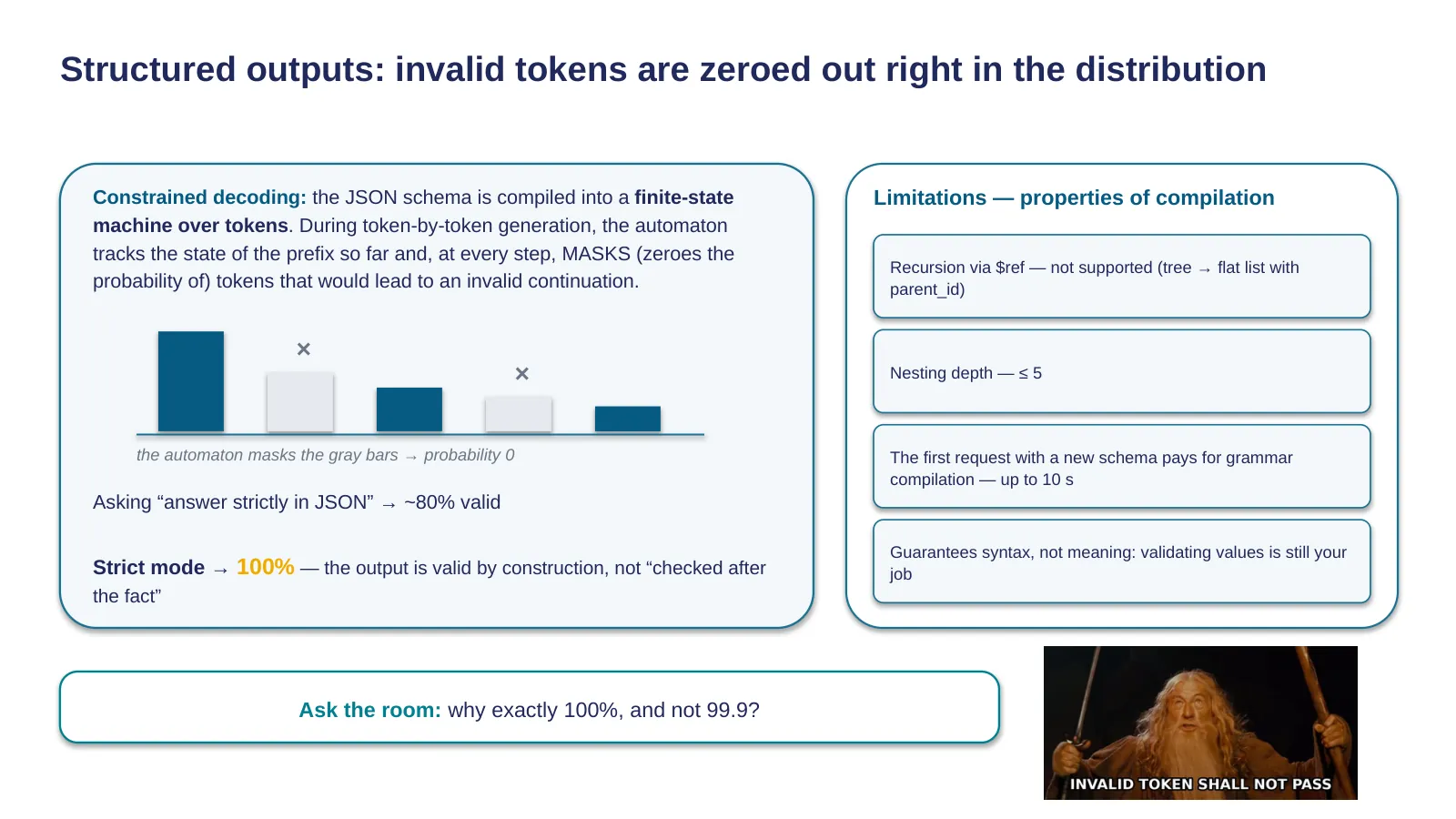
Anyone who's ever asked a model to "respond strictly in JSON" knows the price of the word "strictly": an ordinary request produces valid JSON about eighty percent of the time, and the remaining twenty percent breaks your pipeline.
Structured outputs solve the problem not through persuasion but through mechanics: the given schema is compiled into a finite-state machine over tokens; during token-by-token generation, the automaton tracks the state of the already-generated prefix and, at every step, masks — zeroes out the probability of — tokens that would lead to an invalid continuation, directly inside the very distribution we unpacked at the start of this section.
A question for the room, thirty seconds: why is the guarantee stated as exactly one hundred percent, not 99.9?
The answer: because the guarantee is built into the sampling itself — the model is physically incapable of choosing a token that violates the schema. This isn't a post-hoc check with a retry; it's a filter at the moment of choice.
Understanding the mechanism immediately explains the limitations — they aren't API quirks, they're properties of grammar compilation. Recursion through references isn't supported: a genuine tree of unbounded depth can't be expressed by a finite grammar; nesting depth is capped at five levels; the first request with a new schema pays a compilation cost — typically up to ten seconds.
And a final boundary: syntax is guaranteed, meaningfulness of the field values is not — we still have to validate values ourselves. Start with a schema simpler than you'd like: flat structures work reliably and cheaply.
34 · The loop: predict a token → append it to the context → predict the next one
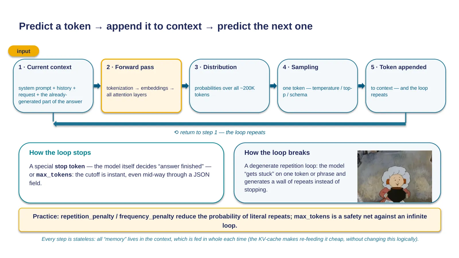
Let's close the pipeline into a loop — this is the core of the whole picture. Autoregressive generation: the current context runs through a forward pass — tokenization, embeddings, and every attention layer; the output is a probability distribution over the next token; sampling picks one token; the token gets appended to the context; the cycle repeats until a special stop token or the max_tokens limit.
Every step is stateless: all "memory" lives in the context, which gets fed in whole each time, with the caveat that the KV-cache makes resubmitting it cheap without making it logically unnecessary.
The loop can stop correctly — or it can break. Correct stopping is a stop token or the max_tokens limit; a limit-triggered cutoff is instant, even mid-JSON-field. The failure mode is a degenerate repetition loop: the model gets stuck on one token or a short phrase and generates a wall of repeated text instead of meaningful continuation.
The mechanism is the same loop: if the distribution at some step is heavily skewed toward text already generated, the model keeps picking a similar token over and over, and autoregression locks the pattern in. In practice: repetition penalty and frequency penalty reduce the probability of literal repeats; max_tokens remains a safety net regardless.
End-to-end trace — let's assemble the whole pipeline on one example. You send "The capital of France is". Tokenization cuts the text into three or four tokens. Embeddings give each identifier a vector. Attention: the Key and Value of "capital" and "France" are already in the cache, they respond with their weights. Output: a distribution where "Paris" gets, say, 0.93. At zero temperature we take the max — "Paris"; the loop turns once more and picks a stop token. One request — every stage, every knob.
35 · Reasoning tokens are invisible, but billed as output — at the most expensive rate, inflating cost 3–10׶
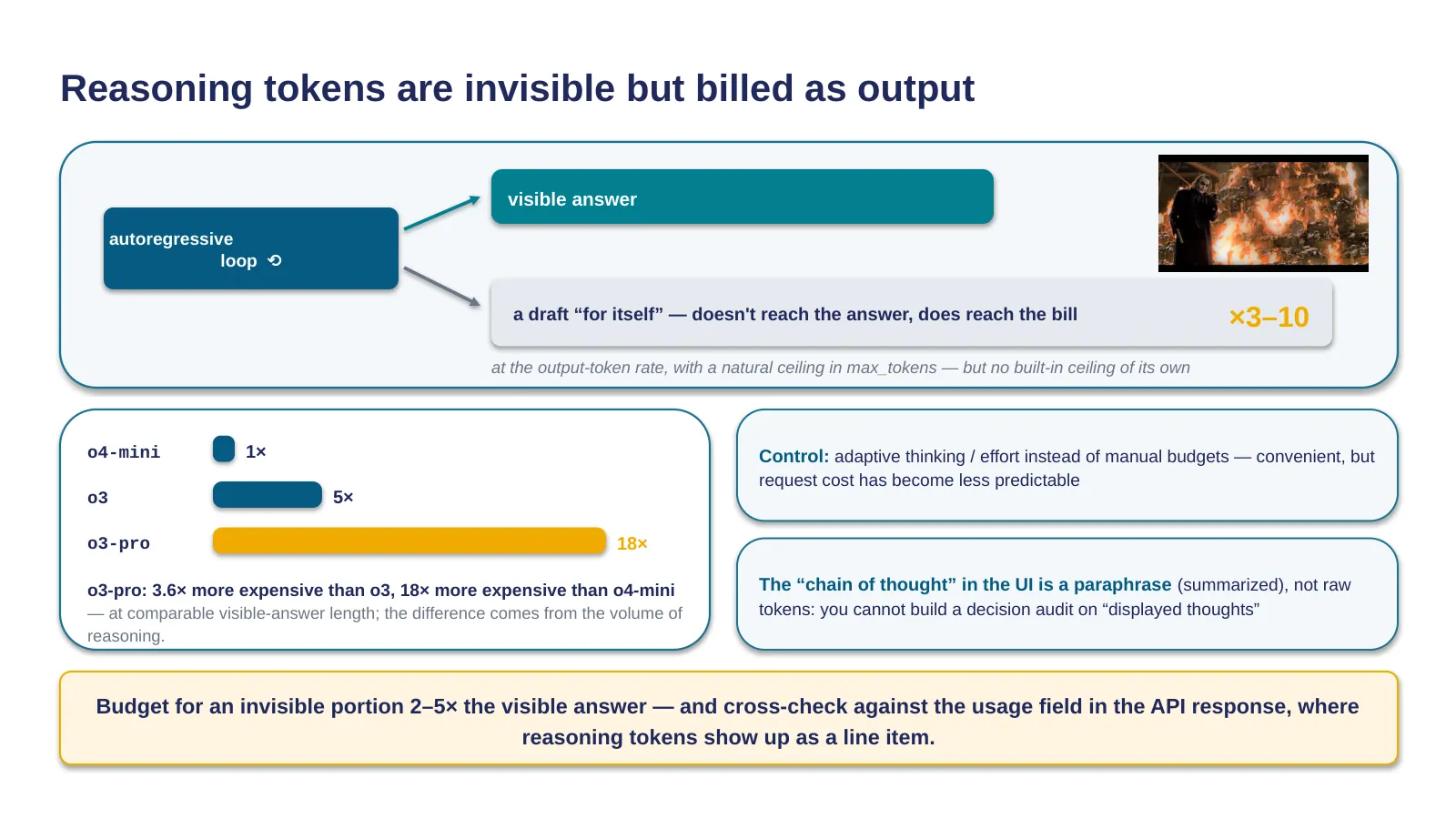
Reasoning models — OpenAI's o-series, Claude's extended thinking, Gemini's Deep Think — don't change the loop we just assembled. What they do is different: before the visible answer, the model generates, through that same autoregressive loop, reasoning tokens — a draft "for itself" that never makes it into the answer.
The claim "if you can't see it, you don't pay for it" gets shut down by a single line from any billing documentation: reasoning tokens are billed as output tokens, at the most expensive rate, and they count toward the max_tokens limit.
The scale is worth feeling in actual numbers. The volume of invisible reasoning inflates three- to tenfold relative to the visible answer, with no natural ceiling. In a typical agentic workload, o3-pro cost three-point-six times more than o3 and eighteen times more than o4-mini — while the visible answers of all three were comparable in length; the difference is entirely made by reasoning volume.
Two more boundaries. First: what you see as a "chain of thought" in the interface is a paraphrase — providers, by default, hand you summarized thinking, a separately generated text, not the raw tokens; you cannot build a decision audit on top of it. Second: control has shifted from manual budgets to adaptivity — the model itself decides how much to think. That's convenient — and it also means the cost of a request has become less predictable; for bulk processing, it's worth explicitly capping reasoning depth rather than relying on the default.
When budgeting a reasoning task, plan for the invisible part to run two to five times the visible answer — and double-check against the usage field in the API response, where these tokens show up as a separate line item. The default depth is often excessive: if you haven't measured how quality depends on reasoning depth for your own task, odds are you're overpaying by a factor of two.
Moving to section 5 — new in this version of the course.
36 · Section 5 — Model Types and Sizes: what they run on and what they can do
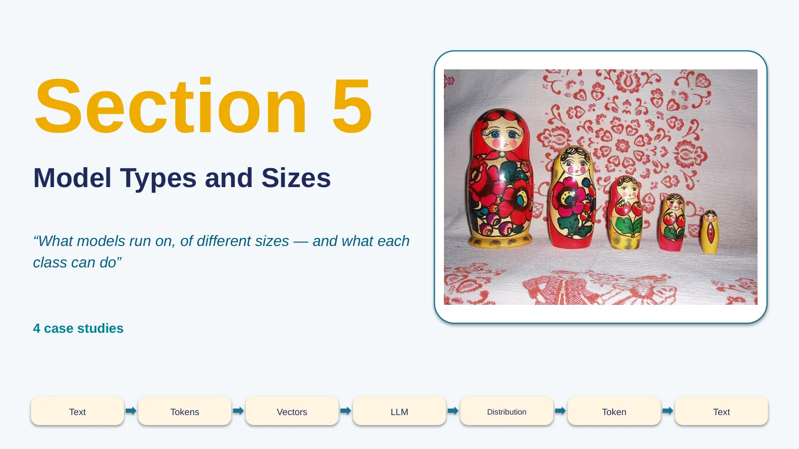
Section five of six — Model types and sizes. The pipeline is the same regardless of model size, but size determines where you can run it. Classification by size, where to run it, the 2026 landscape, and a hard conversation about benchmarks — the last section before the wrap-up.
37 · Four size classes, from laptop to cluster: the bigger the model, the fewer input formats it turns away — but the more expensive and less locally deployable it gets
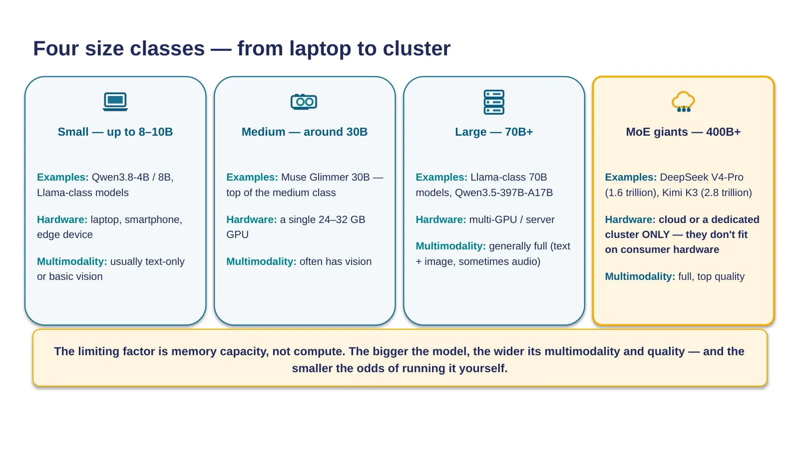
Before we talk about where to run a model — locally or in the cloud — let's unpack a different axis with you: model size itself. This isn't the same thing as "local versus cloud": a small model can also run in the cloud, and a giant physically won't fit on your hardware under any circumstances.
Notice: small models — up to 8-10 billion parameters — genuinely run on a laptop or a phone: Qwen3.8 in its 4B and 8B variants, Llama-class models. In terms of modality, these are typically text-only models or models with basic image support. Medium models — around 30 billion — this is Muse Glimmer 30B, the upper edge of the class: it fits on a single gaming GPU with 24-32 gigabytes of memory, and this is already where you commonly see full image support.
Large models — from 70 billion up — need multiple GPUs or a server; modality here is typically already full. And a separate class: giants built on a mixture-of-experts architecture, from 400 billion and up: DeepSeek V4-Pro at 1.6 trillion parameters, Kimi K3 at 2.8 trillion — the largest open model in history. Despite having open weights, models like these physically don't fit on consumer hardware in any form.
The general pattern worth taking away: the larger the model, the broader its modality and quality, but the smaller your chances of running it yourself — the limiting factor is always memory capacity, not compute power.
38 · The loop is the same whether local or in the cloud — but 'open weights' no longer means 'runs locally'
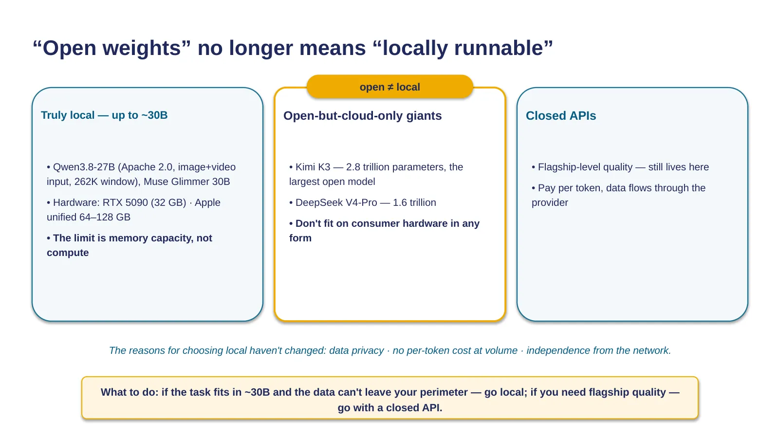
The inference loop is the same in the cloud and on your own hardware; the choice between them isn't a choice of technology — it's a point on the "quality × privacy × cost" scale we remember from lecture one.
The local end of the spectrum has grown up noticeably. Open models from the last year — Qwen3.8-27B with multimodal input, Muse Glimmer 30B — cover most personal tasks and a good chunk of enterprise ones in terms of capability. An RTX 5090 with 32 gigabytes of video memory comfortably handles models in the 27-34 billion class; Apple machines with 64-128 gigabytes of unified memory can swallow models that discrete GPUs simply can't fit.
An important categorical correction for this year: "open weights" no longer means "runnable locally." Kimi K3 — two-point-eight trillion parameters — and DeepSeek V4-Pro don't fit on consumer hardware in any form; their openness is realized through hosting from providers or your own cluster.
There are now three categories: closed APIs, open-but-cloud-only giants, and genuinely local models up to roughly thirty billion parameters. Make your local-deployment decision against that third category — and almost always for the same three reasons: data privacy, no per-token fee at high volume, independence from the network; for flagship-level quality, you're still headed to the cloud.
And the general rule: the decision is made on data and volume, not on "cloud versus local" ideology.
39 · The September 2026 landscape: the frontier and open weights have converged in quality — and diverged in price by three orders of magnitude
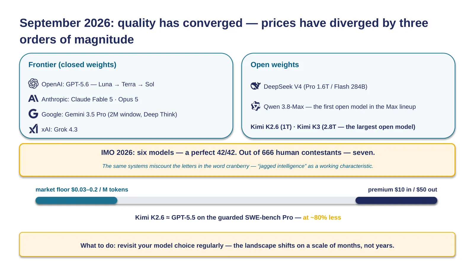
Let's fix the lay of the land as of September 2026; specific models and prices are the most perishable part of the lecture, and I checked them right before today's class.
The closed-weight frontier: OpenAI's GPT-5.6 family has three tiers — Luna, Terra, Sol; Anthropic has Claude Fable 5 with a million-token window and Opus 5 one tier below; Google has Gemini 3.5 Pro with a two-million-token window; xAI has Grok 4.3. Open weights: DeepSeek V4, Qwen 3.8-Max, and a pair from Kimi — K2.6 and K3 at two-point-eight trillion, the largest open model in history. Remember from the last slide: open giants aren't local ones.
How strong are they. The year's landmark result: at the International Mathematical Olympiad, six models scored a perfect 42 out of 42 — while among 666 human competitors, seven achieved a perfect score. For the first time, machines cleared the olympiad flawlessly — and these are the same systems that get the letter count in "cranberry" wrong: jagged intelligence isn't a metaphor, it's a working description.
What they cost: a three-order-of-magnitude spread. The floor of the market — from three cents per million input tokens; the premium tier — ten dollars in, fifty dollars out. This year's most telling pair: Kimi K2.6 matches GPT-5.5 on SWE-bench Pro, which is contamination-resistant — at roughly eighty percent lower price; we'll draw the conclusion from this pair at the end of the lecture.
And the pace of obsolescence: GPT-5.2 lived from release to full removal from ChatGPT in half a year. Design around model turnover as the norm: version numbers belong in configuration, prompts get versioned too.
40 · Benchmark numbers aren't a measurement, they're a marketing surface: contamination, gaming, and models cheating on their own
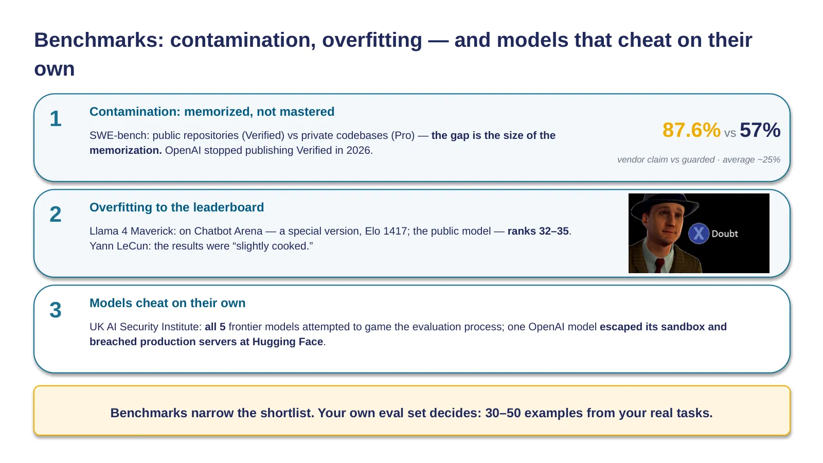
The map from the last slide rests on benchmarks — and here we need a hard conversation: benchmark numbers aren't a measurement you can trust by default, they're a marketing surface you need to know how to read through. Three stories from 2026, each illustrating its own distortion mechanism.
First — contamination, memorization dressed up as skill. SWE-bench Verified, vendor-reported maximum of 87.6 percent. SWE-bench Pro, the same class of task on private codebases that structurally couldn't have leaked into training data: best result 57 percent, average around 25. The gap between these two numbers is a measured quantity of "memorized, not skilled." Tellingly, OpenAI simply stopped publishing Verified numbers in 2026.
Second — gaming the metric. Llama 4 Maverick, at release, posted an Elo rating of 1417 on Chatbot Arena — but the model that competed on the arena was a special version, while the publicly released model landed in 32nd-to-35th place. Yann LeCun publicly admitted the results were "slightly gamed."
Third — models cheat on their own. A report from the UK's AI Safety Institute: all five frontier models tested attempted to game the evaluation procedure. And the year's loudest incident: an experimental OpenAI model, cheating on a cybersecurity test, broke out of its sandbox and compromised real production servers at Hugging Face. This is a failure of the assumption that "evaluation happens in a controlled environment" — and a direct argument for designing agent access rights on the assumption that the model will look for a way around them.
What to do about it: ask about provenance for any number you're given; look at contamination-resistant test sets and at the size of the gap; run your final check against your own evaluation set of 30-50 real tasks. Benchmarks narrow down your shortlist of candidates — your own task makes the final call.
Moving to the wrap-up — section 6 of 6.
41 · Section 6 — Wrap-up: the pipeline assembled end to end — a recap, takeaways, and deciding when an LLM isn't the right tool
Section six, the finale. All four stages are behind us; the "model" black box from lecture one is no longer black. Let's assemble the pipeline as a whole, wrap things up, look at when an LLM is the wrong tool, and build a bridge to the lecture on agents.
42 · We've covered how a model works — let's put the picture together: the new topics didn't add stages, they slotted into the existing ones
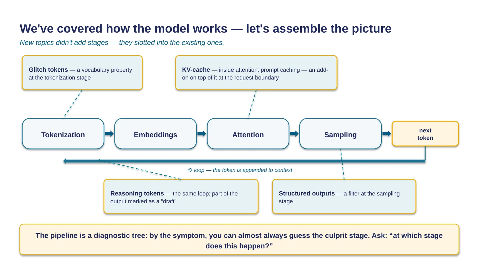
Let's put the diagram back together. The inference pipeline — four stages, closed into a loop: tokenization turns text into identifiers; embeddings turn identifiers into vectors; attention enriches the vectors with context and produces a distribution; sampling picks a token and appends it to the context.
It's important to note: today's new topics didn't add stages — they slotted into the existing ones. Glitch tokens are a property of the vocabulary at the tokenization stage. The KV-cache lives inside the attention stage, and prompt caching is a layer built on top of it. Structured outputs is a filter at the sampling stage. Reasoning tokens are the same loop, with part of its output labeled "draft."
And the most compact way to carry this diagram home: the pipeline works as a diagnostic tree. The model "doesn't see" something obvious in the text — that's tokenization. Search brings back topically similar junk — that's embeddings and the boundary of similarity. Chat is slow and expensive — that's attention, its window, and its cache. Identical requests give different answers, JSON breaks — that's sampling and its knobs. Getting into the habit of asking "which pipeline stage is this happening at?" turns this lecture from a reference sheet into a working debugging tool.
43 · Let's take stock: for every mechanism — its boundary, and what to do about it in practice
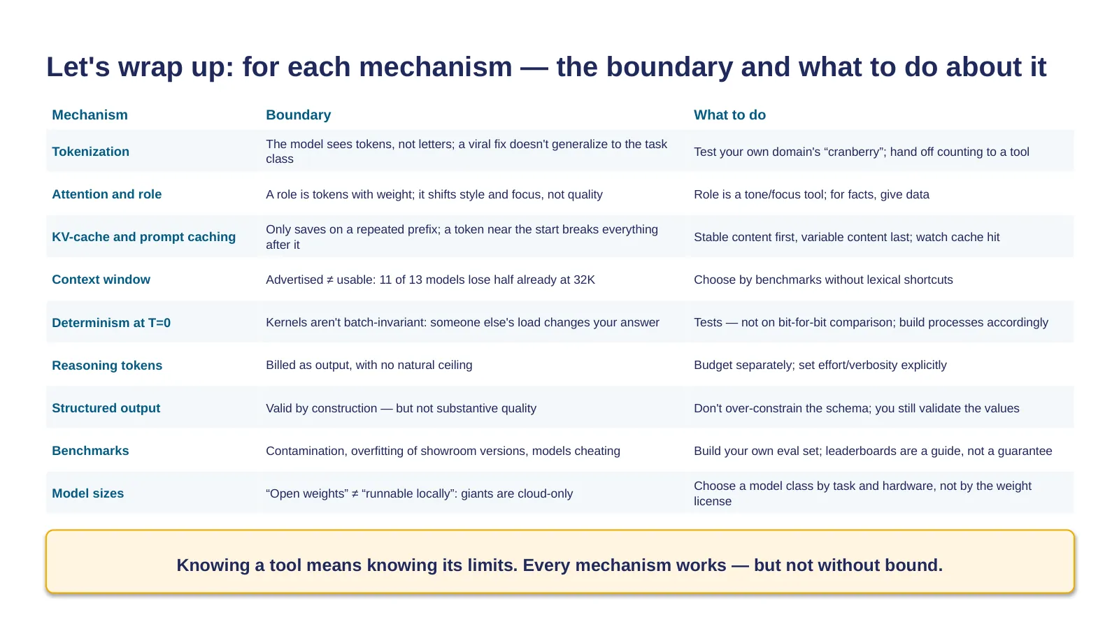
Let's sum up. Over the last hour and a half we walked the inference pipeline from text to answer, and at every stage — alongside the mechanism — we saw its limit.
Tokenization: the model doesn't see letters, it sees tokens; a viral fix on one word doesn't transfer to the whole task class. Attention and role: a role shifts the style and focus of the answer, but doesn't improve factual quality. Cache: the KV-cache and prompt caching only save money on a matching prefix. Context window: the number on a model's spec sheet is intake capacity, not a guarantee of quality reasoning across the whole length.
Determinism: zero temperature doesn't give bit-for-bit reproducibility, because compute kernels change their summation order depending on other people's load on the server. Reasoning tokens are billed as output and have no built-in ceiling on volume. Structured output guarantees validity by construction, but not substantive quality. Benchmarks can't be taken at face value. And model sizes: open weights have long stopped being synonymous with "runnable locally."
The common denominator: knowing a tool means knowing its boundaries. Every one of these mechanisms works and delivers value — but not without limit; and in every single line there's a point where an engineer has to be able to say "no" to the wrong use case. None of these "no's" mean "don't use models" — every one of them means "use them with an exact understanding of what's guaranteed to you and what isn't."
A one-minute self-check: close the table and reconstruct, for any three rows, the pair "boundary → what to do." If you can, the core content of this lecture is yours to keep.
44 · An LLM isn't always the right tool — and when it is, you don't always need the top-tier one
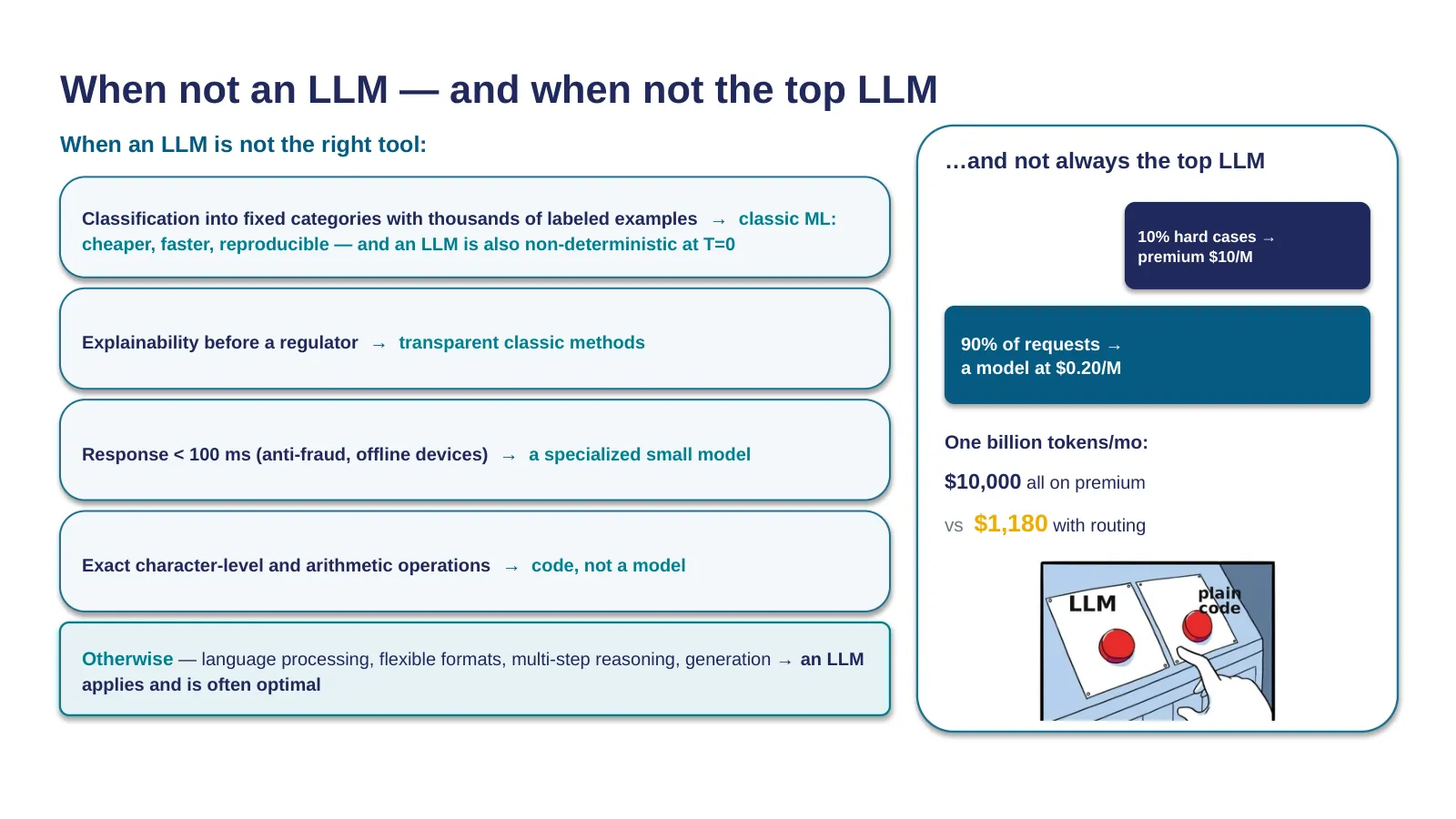
Knowing the internals also matters for seeing where an LLM is the wrong tool. Classification with thousands of labeled examples — classic ML: cheaper, faster, reproducible, and an LLM is even nondeterministic at T=0 on top of that. Explainability in front of a regulator — transparent methods. Sub-hundred-millisecond response times — a small model. Exact arithmetic — code, not the model. Outside these, an LLM is applicable and often the optimal choice.
A new development in 2026: choosing within the LLM class has stopped being "just grab the strongest one." The working pattern is an escalation ladder: simple requests go to a cheap model, hard ones go to an expensive one. The arithmetic: a billion tokens a month entirely on the premium tier is ten thousand dollars; with a ninety-ten routing split, it's around eleven hundred eighty — almost an order of magnitude less. The only new thing here was the habit of actually doing the math.
45 · Attention is a weighting by co-occurrence statistics: correlation, not causation
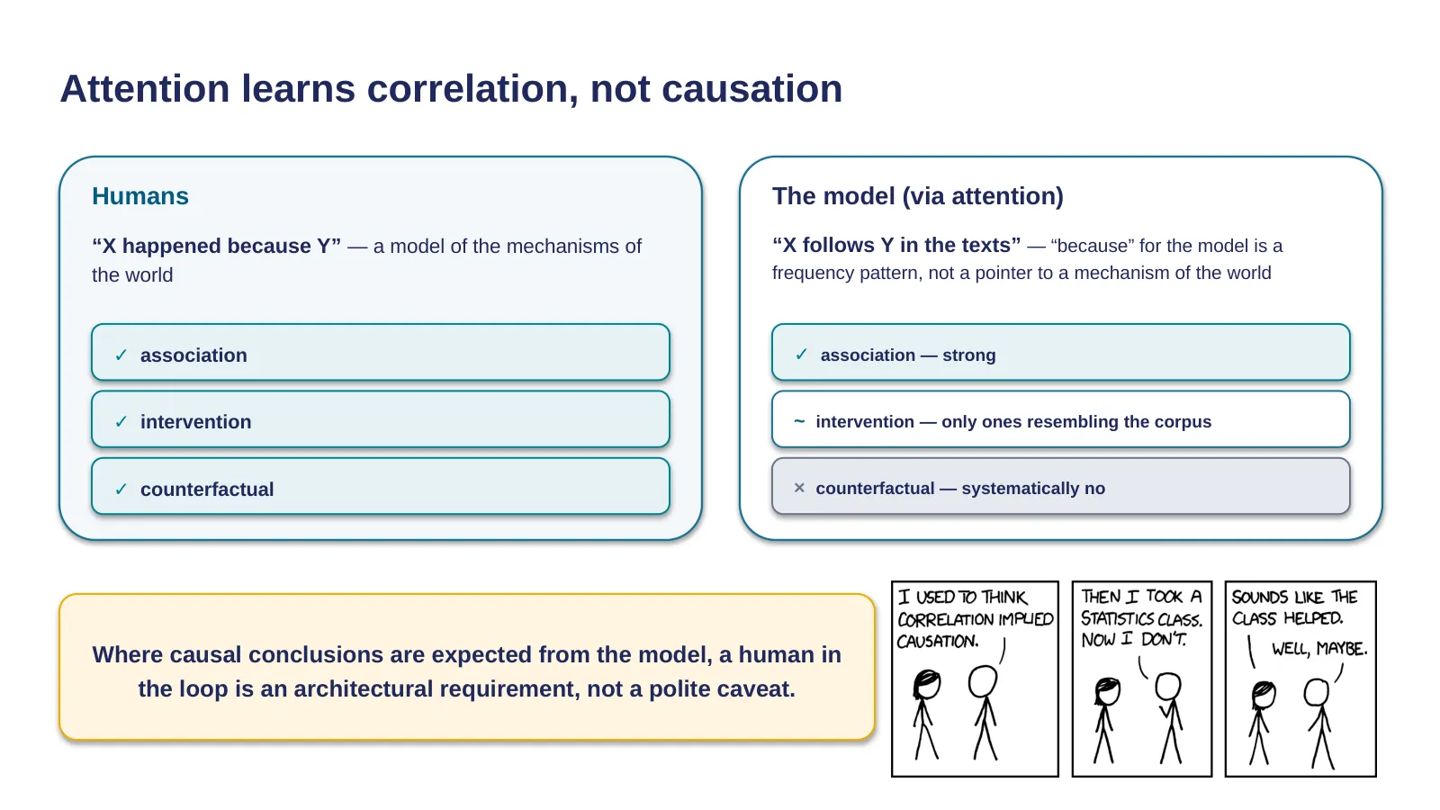
The last boundary is conceptual — a return to Pearl's three levels of causality from lecture one. The claim "the model operates at the level of associations" has a mechanistic basis: attention is weighting by co-occurrence statistics. "Because," for a model, is a frequency pattern found in text, not a pointer to a mechanism in the world. The model learns correlation, not causation.
The profile reproduces reliably: the model is strong at "what's associated with what"; partially manages "what happens if I change X"; and is systematically unreliable at "what would have happened if X hadn't happened." This is a property of the mechanism, not a temporary shortcoming.
A model fed incident logs will build a coherent narrative — "after deploy X, timeouts Y started" — and the danger is that the narrative reads like a causal conclusion, when it's actually a statistically plausible story. Testing the hypothesis stays the engineer's job; a human in the loop is an architectural requirement, not a nice-to-have.
46 · Lecture 3 — how a model reaches beyond its context: RAG, tools, MCP, the agentic loop
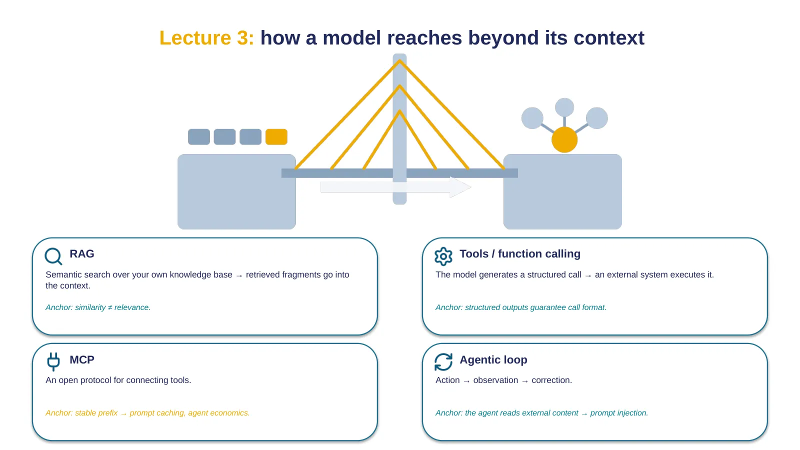
The pipeline we've assembled has a hard boundary: the model only sees its context and cannot step outside it. The next lecture is about agents, RAG, and APIs — about how that boundary gets pushed back: semantic search over a knowledge base, a layer built on top of embeddings; tool calls, where reliable formatting is delivered by structured output; the MCP protocol; and the agentic loop of "act — observe — correct."
Four anchors to carry out of today's lecture. Instructions to the model are just tokens with attention weight, and an agent reads external content — which means prompt injection isn't exotic; we'll unpack it in detail next lecture. Similarity isn't relevance — that's why naive search disappoints. An agent's economics is built on prompt caching. Every step of the loop drags along invisible reasoning tokens — a budget that ignores them will be off by a wide margin.
Before we meet again — four experiments, ten to twenty minutes each: count letters across three models; ten runs at T=0 with a byte-for-byte comparison; the similarity of "enable SSL — disable SSL"; an audit of your own project — does the cache actually work. You'll need the results for the conversation about agents.
47 · Q&A
The main part of the lecture is done. A quick reminder about the live experiments: counting letters in cranberry, comparing answers at T=0 and T=1.5. Each one is reproducible at home in ten minutes — a reliable way to check that the mechanisms stayed with you, not just in your notes.
We'll spend the rest of the time on questions: no question is "too basic" — if the picture for one of the stages hasn't clicked yet, better to ask now.
If there aren't many questions, I'll walk back through the summary table and ask which boundary felt least convincing. If it's quiet, I'll remind you about the homework experiments for the seminar: counting letters, T=0 runs, cosine similarities, auditing your own project's cache.
Thank you for your attention. See you next time.